Example: Helix active wake mixing

"""Example: Helix active wake mixing

Example to test out using helix wake mixing of upstream turbines.
Helix wake mixing is turned on at turbine 1, off at turbines 2 to 4;
Turbine 2 is in wake turbine 1, turbine 4 in wake of turbine 3.
"""

import matplotlib.pyplot as plt
import numpy as np
import yaml

import floris.flow_visualization as flowviz
from floris import FlorisModel


# Grab model of FLORIS and update to awc-enabled turbines
fmodel = FlorisModel("../inputs/emgauss_helix.yaml")
fmodel.set_operation_model("awc")

# Set the wind directions and speeds to be constant over N different helix amplitudes
N = 1
awc_modes = np.array(["helix", "baseline", "baseline", "baseline"]).reshape(4, N).T
awc_amplitudes = np.array([2.5, 0, 0, 0]).reshape(4, N).T

# Create 4 WT WF layout with lateral offset of 3D and streamwise offset of 4D
D = 240
fmodel.set(
    layout_x=[0.0, 4*D, 0.0, 4*D],
    layout_y=[0.0, 0.0, -3*D, -3*D],
    wind_directions=270 * np.ones(N),
    wind_speeds=8.0 * np.ones(N),
    turbulence_intensities=0.06*np.ones(N),
    awc_modes=awc_modes,
    awc_amplitudes=awc_amplitudes
)
fmodel.run()
turbine_powers = fmodel.get_turbine_powers()

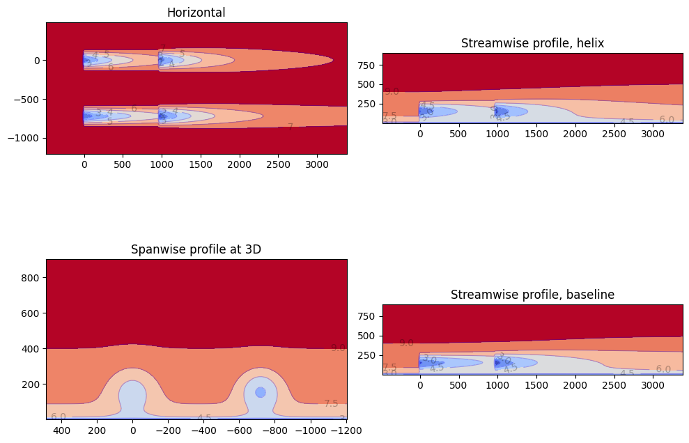
# Plot the flow fields for T1 awc_amplitude = 2.5
horizontal_plane = fmodel.calculate_horizontal_plane(
    x_resolution=200,
    y_resolution=100,
    height=150.0,
)

y_plane_baseline = fmodel.calculate_y_plane(
    x_resolution=200,
    z_resolution=100,
    crossstream_dist=0.0,
)
y_plane_helix = fmodel.calculate_y_plane(
    x_resolution=200,
    z_resolution=100,
    crossstream_dist=-3*D,
)

cross_plane = fmodel.calculate_cross_plane(
    y_resolution=100,
    z_resolution=100,
    downstream_dist=720.0,
)

# Create the plots
fig, ax_list = plt.subplots(2, 2, figsize=(10, 8), tight_layout=True)
ax_list = ax_list.flatten()
flowviz.visualize_cut_plane(
    horizontal_plane,
    ax=ax_list[0],
    label_contours=True,
    title="Horizontal"
)
flowviz.visualize_cut_plane(
    cross_plane,
    ax=ax_list[2],
    label_contours=True,
    title="Spanwise profile at 3D"
)

# fig2, ax_list2 = plt.subplots(2, 1, figsize=(10, 8), tight_layout=True)
# ax_list2 = ax_list2.flatten()
flowviz.visualize_cut_plane(
    y_plane_baseline,
    ax=ax_list[1],
    label_contours=True,
    title="Streamwise profile, helix"
)
flowviz.visualize_cut_plane(
    y_plane_helix,
    ax=ax_list[3],
    label_contours=True,
    title="Streamwise profile, baseline"
)

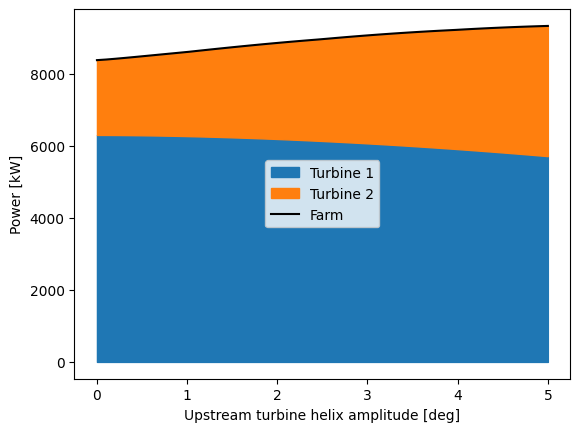
# Calculate the effect of changing awc_amplitudes
N = 50
awc_amplitudes = np.array([
    np.linspace(0, 5, N),
    np.zeros(N), np.zeros(N), np.zeros(N)
    ]).reshape(4, N).T

# Reset FlorisModel for different helix amplitudes
fmodel.set(
    wind_directions=270 * np.ones(N),
    wind_speeds=8 * np.ones(N),
    turbulence_intensities=0.06*np.ones(N),
    awc_modes=awc_modes,
    awc_amplitudes=awc_amplitudes
    )
fmodel.run()
turbine_powers = fmodel.get_turbine_powers()

# Plot the power as a function of helix amplitude
fig_power, ax_power = plt.subplots()
ax_power.fill_between(
    awc_amplitudes[:, 0],
    0,
    turbine_powers[:, 0]/1000,
    color='C0',
    label='Turbine 1'
    )
ax_power.fill_between(
    awc_amplitudes[:, 0],
    turbine_powers[:, 0]/1000,
    turbine_powers[:, :2].sum(axis=1)/1000,
    color='C1',
    label='Turbine 2'
    )
ax_power.plot(
    awc_amplitudes[:, 0],
    turbine_powers[:,:2].sum(axis=1)/1000,
    color='k',
    label='Farm'
    )

ax_power.set_xlabel("Upstream turbine helix amplitude [deg]")
ax_power.set_ylabel("Power [kW]")
ax_power.legend()

flowviz.show()
import warnings
warnings.filterwarnings('ignore')