Example 3: Wind Data Objects

"""Example 3: Wind Data Objects

This example demonstrates the use of wind data objects in FLORIS:
 TimeSeries, WindRose, and WindTIRose.

 For each of the WindData objects, examples are shown of:

    1) Initializing the object
    2) Broadcasting values
    3) Converting between objects
    4) Setting TI and value
    5) Plotting
    6) Setting the FLORIS model using the object

"""


import matplotlib.pyplot as plt
import numpy as np

from floris import (
    FlorisModel,
    TimeSeries,
    WindRose,
    WindTIRose,
)


##################################################
# Initializing
##################################################

# FLORIS provides a set of wind data objects to hold the ambient wind conditions in a
# convenient classes that include capabilities and methods to manipulate and visualize
# the data.

# The TimeSeries class is used to hold time series data, such as wind speed, wind direction,
# and turbulence intensity.

# There is also a "value" wind data variable, which represents the value of the power
# generated at each time step or wind condition (e.g., the price of electricity). This can
# then be used in later optimization methods to optimize for quantities besides AEP.

# Generate wind speeds, directions, turbulence intensities, and values via random signals
N = 100
wind_speeds = 8 + 2 * np.random.randn(N)
wind_directions = 270 + 30 * np.random.randn(N)
turbulence_intensities = 0.06 + 0.02 * np.random.randn(N)
values = 25 + 10 * np.random.randn(N)

time_series = TimeSeries(
    wind_directions=wind_directions,
    wind_speeds=wind_speeds,
    turbulence_intensities=turbulence_intensities,
    values=values,
)

# The WindRose class is used to hold wind rose data, such as wind speed, wind direction,
# and frequency.  TI and value are represented as bin averages per wind direction and
# speed bin.
wind_directions = np.arange(0, 360, 3.0)
wind_speeds = np.arange(4, 20, 2.0)

# Make TI table 6% TI for all wind directions and speeds
ti_table = 0.06 * np.ones((len(wind_directions), len(wind_speeds)))

# Make value table 25 for all wind directions and speeds
value_table =25 * np.ones((len(wind_directions), len(wind_speeds)))

# Uniform frequency
freq_table = np.ones((len(wind_directions), len(wind_speeds)))
freq_table = freq_table / np.sum(freq_table)

wind_rose = WindRose(
    wind_directions=wind_directions,
    wind_speeds=wind_speeds,
    ti_table=ti_table,
    freq_table=freq_table,
    value_table=value_table,
)

# The WindTIRose class is similar to the WindRose table except that TI is also binned
# making the frequency table a 3D array.
turbulence_intensities = np.arange(0.05, 0.15, 0.01)

# Uniform frequency
freq_table = np.ones((len(wind_directions), len(wind_speeds), len(turbulence_intensities)))

# Uniform value
value_table = 25* np.ones((len(wind_directions), len(wind_speeds), len(turbulence_intensities)))

wind_ti_rose = WindTIRose(
    wind_directions=wind_directions,
    wind_speeds=wind_speeds,
    turbulence_intensities=turbulence_intensities,
    freq_table=freq_table,
    value_table=value_table,
)

##################################################
# Broadcasting
##################################################

# A convenience method of the wind data objects is that, unlike the lower-level
# FlorisModel.set() method, the wind data objects can broadcast upward data provided
# as a scalar to the full array.  This is useful for setting the same wind conditions
# for all turbines in a wind farm.

# For TimeSeries, as long as one condition is given as an array, the other 2
# conditions can be given as scalars.  The TimeSeries object will broadcast the
# scalars to the full array (uniform)
wind_directions = 270 + 30 * np.random.randn(N)
time_series = TimeSeries(
    wind_directions=wind_directions, wind_speeds=8.0, turbulence_intensities=0.06
)


# For WindRose, wind directions and wind speeds must be given as arrays, but the
# ti_table can be supplied as a scalar which will apply uniformly to all wind
# directions and speeds.  Not supplying a freq table will similarly generate
# a uniform frequency table.
wind_directions = np.arange(0, 360, 3.0)
wind_speeds = np.arange(4, 20, 2.0)
wind_rose = WindRose(wind_directions=wind_directions, wind_speeds=wind_speeds, ti_table=0.06)


##################################################
# Wind Rose from Time Series
##################################################

# The TimeSeries class has a method to generate a wind rose from a time series based on binning
wind_rose = time_series.to_WindRose(wd_edges=np.arange(0, 360, 3.0), ws_edges=np.arange(2, 20, 2.0))

##################################################
# Wind Rose from long CSV FILE
##################################################

# The WindRose class can also be initialized from a long CSV file.  By long what is meant is
# that the file has a column for each wind direction, wind speed combination.  The file can
# also specify the mean TI per bin and the frequency of each bin as seperate columns.

# If the TI is not provided, can specify a fixed TI for all bins using the ti_col_or_value
# input
wind_rose_from_csv = WindRose.read_csv_long(
    "inputs/wind_rose.csv", wd_col="wd", ws_col="ws", freq_col="freq_val", ti_col_or_value=0.06
)

##################################################
# Aggregating and Resampling the Wind Rose
##################################################

# The aggregate function allows for aggregation of the wind rose data into
# fewer wind direction and wind speed bins.
# Note it will throw an error if the step sizes passed in are smaller than the
# step sizes of the original data.
wind_rose_aggregate = wind_rose.aggregate(wd_step=10, ws_step=2)

# For upsampling, the resample_by_interpolation function can be used to interpolate
# the wind rose data to a finer grid.  It can use either linear or nearest neighbor
wind_rose_resample = wind_rose.resample_by_interpolation(wd_step=0.5, ws_step=0.25)

##################################################
# Setting turbulence intensity
##################################################

# Each of the wind data objects also has the ability to set the turbulence intensity
# according to a function of wind speed and direction.  This can be done using a custom
# function by using the assign_ti_using_wd_ws_function method. There is also a method
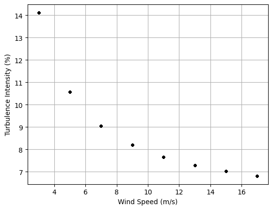
# called assign_ti_using_IEC_method which assigns TI based on the IEC 61400-1 standard.
wind_rose.assign_ti_using_IEC_method()  # Assign using default settings for Iref and offset

##################################################
# Setting value
##################################################

# Similarly, each of the wind data objects also has the ability to set the value according to
# a function of wind speed and direction.  This can be done using a custom function by using
# the assign_value_using_wd_ws_function method. There is also a method called
# assign_value_piecewise_linear which assigns value based on a linear piecewise function of
# wind speed.

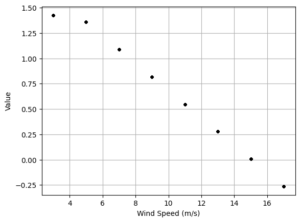
# Assign value using default settings. This produces a value vs. wind speed that approximates
# the normalized mean electricity price vs. wind speed curve for the SPP market in the U.S.
# for years 2018-2020 from figure 7 in "The value of wake steering wind farm flow control in
# US energy markets," Wind Energy Science, 2024. https://doi.org/10.5194/wes-9-219-2024.
wind_rose.assign_value_piecewise_linear()

##################################################
# Plotting Wind Data Objects
##################################################

# Certain plotting methods are included to enable visualization of the wind data objects
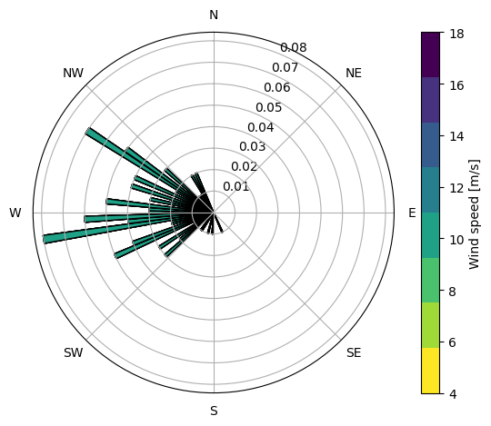
# Plotting a wind rose
wind_rose.plot()

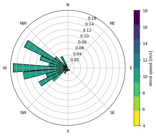
# Plot a wind rose with the wind directions aggregated into 10-deg bins
wind_rose.plot(wd_step=10)

# Showing TI over wind speed for a WindRose
wind_rose.plot_ti_over_ws()

# Showing value over wind speed for a WindRose
wind_rose.plot_value_over_ws()

##################################################
# Setting the FLORIS model via wind data
##################################################

# Each of the wind data objects can be used to set the FLORIS model by passing
# them in as is to the set method.  The FLORIS model will then use the member functions
# of the wind data to extract the wind conditions for the simulation.  Frequency tables
# are also extracted for expected power and AEP-like calculations.
# Similarly the value data is extracted and maintained.

fmodel = FlorisModel("inputs/gch.yaml")

# Set the wind conditions using the TimeSeries object
fmodel.set(wind_data=time_series)

# Set the wind conditions using the WindRose object
fmodel.set(wind_data=wind_rose)

# Note that in the case of the wind_rose, under the default settings, wind direction and wind speed
# bins for which frequency is zero are not simulated.  This can be changed by setting the
# compute_zero_freq_occurrence parameter to True.
wind_directions = np.array([200.0, 300.0])
wind_speeds = np.array([5.0, 1.00])
freq_table = np.array([[0.5, 0], [0.5, 0]])
wind_rose = WindRose(
    wind_directions=wind_directions, wind_speeds=wind_speeds, ti_table=0.06, freq_table=freq_table
)
fmodel.set(wind_data=wind_rose)

print(
    f"Number of conditions to simulate with compute_zero_freq_occurrence = False: "
    f"{fmodel.n_findex}"
)

wind_rose = WindRose(
    wind_directions=wind_directions,
    wind_speeds=wind_speeds,
    ti_table=0.06,
    freq_table=freq_table,
    compute_zero_freq_occurrence=True,
)
fmodel.set(wind_data=wind_rose)

print(
    f"Number of conditions to simulate with compute_zero_freq_occurrence = "
    f"True: {fmodel.n_findex}"
)

# Set the wind conditions using the WindTIRose object
fmodel.set(wind_data=wind_ti_rose)

plt.show()
import warnings
warnings.filterwarnings('ignore')

Number of conditions to simulate with compute_zero_freq_occurrence = False: 2
Number of conditions to simulate with compute_zero_freq_occurrence = True: 4