Example: Layout optimization with WindRoseWRG comparison#
"""Example: Layout optimization with WindRoseWRG comparison
This example compares a layout optimization using a WindRoseWRG. In the example, two
turbine positions are optimized within a square grid. The optimization is run 3 times:
1. Using a WindRoseWRG object generated using the example wrg file
2. Using a WindRose object created from the WindRoseWRG object
3. Using a WindRose object created from the WindRoseWRG object, but with the HeterogeneousMap
also generated by the WindRoseWRG object
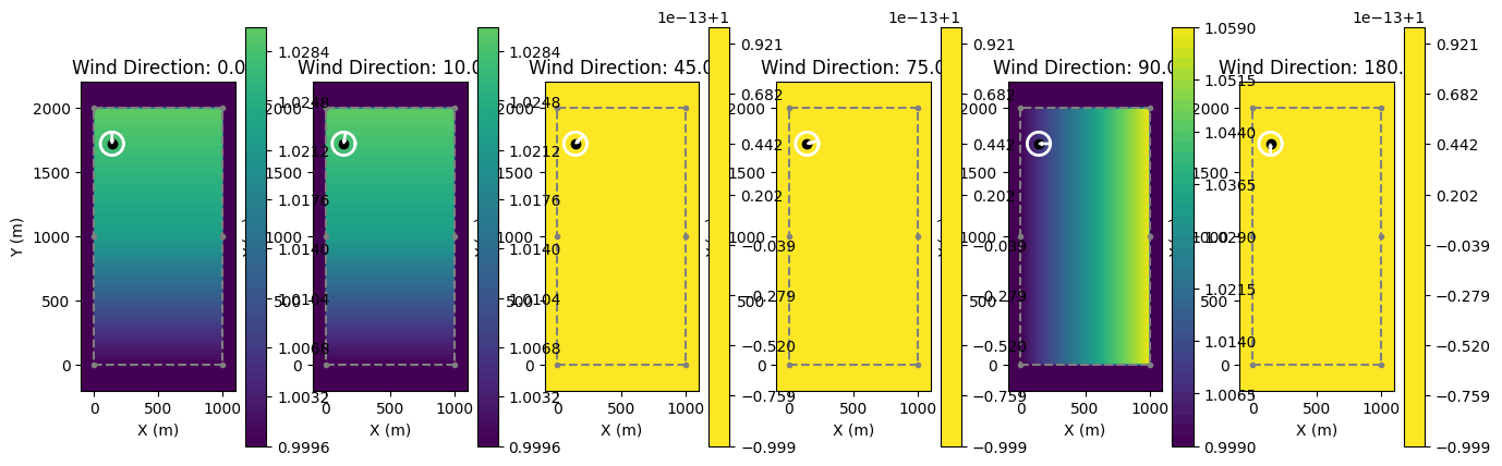
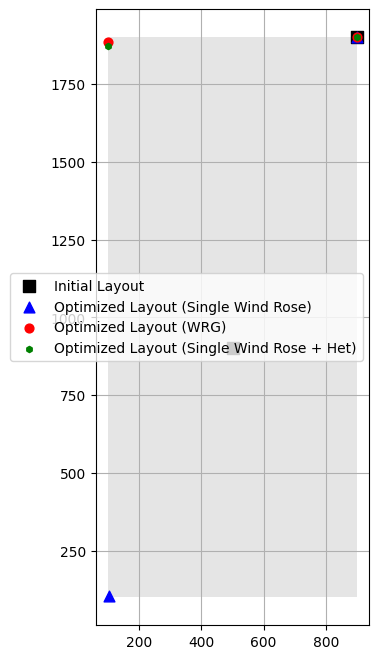
Because the WRG file includes a speed-up for northern winds, optimizaitions (1) and (3) place both
turbines near the northern boundary of the grid, while optimization (2) places the turbines in the
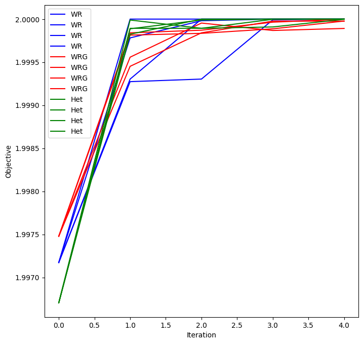
furthest corners of the grid. The optimization illustrates that using the full WindRoseWRG object
produces a similar result to the WindRose object with the HeterogeneousMap, since they both
can represent the difference in resource for different locations. The HeterogeneousMap may have
advantage for larger cases since it is running with only 1 wind speed. For this example the results
and performance are similar.
"""
import matplotlib.pyplot as plt
import numpy as np
from floris import (
FlorisModel,
WindRoseWRG,
)
from floris.optimization.layout_optimization.layout_optimization_random_search import (
LayoutOptimizationRandomSearch,
)
if __name__ == "__main__":
# Parameters of layout optimization
seconds_per_iteration = 30.0
total_optimization_seconds = 120.0
min_dist_D = 3.0
use_dist_based_init = False
# Initialize the WindRoseWRG object with wind speeds every 2 m/s and fixed ti of 6%. Specify
# a wd_step of 4 degrees, which implies upsampling from wrg's 90 degree sectors to 12
# degree sectors
wind_rose_wrg = WindRoseWRG(
"wrg_example.wrg",
wd_step=2.0,
wind_speeds=np.arange(0, 21, 1.0), # Use a sparser range of speeds
ti_table=0.06,
)
# Define an optimization boundary within the grid that is a square with a
# buffer to avoid the outer limits of the heterogeneous area
buffer = 100.0
boundaries = [
(buffer, buffer),
(1000 - buffer, buffer),
(1000 - buffer, 2000 - buffer),
(buffer, 2000 - buffer),
(buffer, buffer),
]
# Select and initial layout in the corners of the boundary
layout_x = np.array([500, 1000 - buffer])
layout_y = np.array([900, 2000 - buffer])
##########################
# Set up the FlorisModel
fmodel = FlorisModel("../inputs/gch.yaml")
##########################
# Use the get_heterogeneous_map method to generate a WindRose that represents
# the information in the WindRoseWRG, rather than a set of WindRose objects
# but as a single WindRose object (for one location) and a HeterogeneousMap
# the describes the speed up information per direction across the domain
# This will allow running the optimization for a single wind speed while still
# accounting for the difference in wind speeds in location by direction
wind_rose_het = wind_rose_wrg.get_heterogeneous_wind_rose(
fmodel=fmodel,
x_loc=0.0,
y_loc=0.0,
representative_wind_speed=9.0,
)
# Pull out the heterogeneous plot to show the underlying speedups
het_map = wind_rose_het.heterogeneous_map
wind_direction_to_plot = [0.0, 10.0, 45.0, 75.0, 90.0, 180.0]
# Show the het_map for a few wind directions
fig, axarr = plt.subplots(1, len(wind_direction_to_plot), figsize=(16, 5))
axarr = axarr.flatten()
for i, wd in enumerate(wind_direction_to_plot):
het_map.plot_single_speed_multiplier(
wind_direction=wd,
wind_speed=8.0,
ax=axarr[i],
show_colorbar=True,
)
axarr[i].set_title(f"Wind Direction: {wd}")
# ##########################
# Run the optimization with the full WindRoseWRG first
fmodel.set(layout_x=layout_x, layout_y=layout_y, wind_data=wind_rose_wrg)
# Set the layout optimization
layout_opt = LayoutOptimizationRandomSearch(
fmodel,
boundaries,
min_dist_D=min_dist_D,
seconds_per_iteration=seconds_per_iteration,
total_optimization_seconds=total_optimization_seconds,
use_dist_based_init=use_dist_based_init,
)
layout_opt.optimize()
x_initial, y_initial, x_opt_wrg, y_opt_wrg = layout_opt._get_initial_and_final_locs()
# Grab the log array
objective_log_array_wrg = np.array(layout_opt.objective_candidate_log)
# Normalize
objective_log_array_wrg = objective_log_array_wrg / np.max(objective_log_array_wrg)
print("=====================================")
print("Objective log array (WRG):")
print(objective_log_array_wrg.shape)
print(objective_log_array_wrg)
# ##########################
# Repeat using wind_rose_het
fmodel.set(layout_x=layout_x, layout_y=layout_y, wind_data=wind_rose_het)
# Set the layout optimization
layout_opt = LayoutOptimizationRandomSearch(
fmodel,
boundaries,
min_dist_D=min_dist_D,
seconds_per_iteration=seconds_per_iteration,
total_optimization_seconds=total_optimization_seconds,
use_dist_based_init=use_dist_based_init,
)
layout_opt.optimize()
_, _, x_opt_het, y_opt_het = layout_opt._get_initial_and_final_locs()
# Grab the log array
objective_log_array_het = np.array(layout_opt.objective_candidate_log)
# Normalize
objective_log_array_het = objective_log_array_het / np.max(objective_log_array_het)
# ##########################
# Repeat using single wind rose (without het)
wind_rose = wind_rose_wrg.get_wind_rose_at_point(0, 0)
fmodel = FlorisModel("../inputs/gch.yaml")
fmodel.set(layout_x=layout_x, layout_y=layout_y, wind_data=wind_rose)
# Set the layout optimization
layout_opt = LayoutOptimizationRandomSearch(
fmodel,
boundaries,
min_dist_D=min_dist_D,
seconds_per_iteration=seconds_per_iteration,
total_optimization_seconds=total_optimization_seconds,
use_dist_based_init=use_dist_based_init,
)
layout_opt.optimize()
_, _, x_opt_wr, y_opt_wr = layout_opt._get_initial_and_final_locs()
# Grab the log array
objective_log_array_wr = np.array(layout_opt.objective_candidate_log)
# Normalize
objective_log_array_wr = objective_log_array_wr / np.max(objective_log_array_wr)
fig, ax = plt.subplots(1, 1, figsize=(8, 8))
layout_opt.plot_layout_opt_boundary(ax=ax)
ax.scatter(x_initial, y_initial, label="Initial Layout", s=80, color="k", marker="s")
ax.scatter(
x_opt_wr, y_opt_wr, label="Optimized Layout (Single Wind Rose)", s=60, color="b", marker="^"
)
ax.scatter(x_opt_wrg, y_opt_wrg, label="Optimized Layout (WRG)", s=40, color="r", marker="o")
ax.scatter(
x_opt_het,
y_opt_het,
label="Optimized Layout (Single Wind Rose + Het)",
s=20,
color="g",
marker="h",
)
ax.set_aspect('equal')
ax.legend()
print("=====================================")
print("Objective log array (HET):")
print(objective_log_array_het.shape)
print(objective_log_array_het)
fig, ax = plt.subplots(1, 1, figsize=(8, 8))
for objective_log_array, label, color in zip(
[objective_log_array_wr, objective_log_array_wrg, objective_log_array_het],
["WR", "WRG", "Het"],
["b", "r", "g"],
):
ax.plot(
np.arange(len(objective_log_array)),
np.log10(objective_log_array * 100.0),
label=label,
color=color,
)
ax.set_xlabel("Iteration")
ax.set_ylabel("Objective")
ax.legend()
plt.show()
import warnings
warnings.filterwarnings('ignore')
/home/runner/work/floris/floris/floris/core/flow_field.py:169: UserWarning: 'where' used without 'out', expect unitialized memory in output. If this is intentional, use out=None.
  * np.power(
/home/runner/work/floris/floris/floris/core/wake_deflection/gauss.py:325: RuntimeWarning: invalid value encountered in divide
  val = 2 * (avg_v - v_core) / (v_top + v_bottom)
/home/runner/work/floris/floris/floris/core/wake_deflection/gauss.py:160: RuntimeWarning: invalid value encountered in divide
  C0 = 1 - u0 / freestream_velocity
/home/runner/work/floris/floris/floris/core/wake_velocity/gauss.py:80: RuntimeWarning: invalid value encountered in divide
  sigma_z0 = rotor_diameter_i * 0.5 * np.sqrt(uR / (u_initial + u0))
/home/runner/work/floris/floris/floris/wind_data.py:3088: RuntimeWarning: invalid value encountered in power
  exponent = -((x / a) ** k)
Using point 0 at (0.0, 0.0) as reference location
/home/runner/work/floris/floris/floris/core/wake_deflection/gauss.py:495: RuntimeWarning: invalid value encountered in divide
  I_total = np.sqrt((2 / 3) * k_total) / average_u_i
Using supplied initial layout for 4 individuals.
=======================================
Optimization step +0.0
Optimization time = +0.0 [s]
Mean AEP = 40.6 [GWh] (+0.00%)
Median AEP = 40.6 [GWh] (+0.00%)
Max AEP = 40.6 [GWh] (+0.00%)
Min AEP = 40.6 [GWh] (+0.00%)
=======================================
Optimizing using 4 individuals.
Optimization time: 0.0 s / 120.0 s
/home/runner/work/floris/floris/floris/wind_data.py:3088: RuntimeWarning: invalid value encountered in power
  exponent = -((x / a) ** k)
/home/runner/work/floris/floris/floris/wind_data.py:3088: RuntimeWarning: invalid value encountered in power
  exponent = -((x / a) ** k)
/home/runner/work/floris/floris/floris/wind_data.py:3088: RuntimeWarning: invalid value encountered in power
  exponent = -((x / a) ** k)
/home/runner/work/floris/floris/floris/wind_data.py:3088: RuntimeWarning: invalid value encountered in power
  exponent = -((x / a) ** k)
/home/runner/work/floris/floris/floris/core/flow_field.py:169: UserWarning: 'where' used without 'out', expect unitialized memory in output. If this is intentional, use out=None.
  * np.power(
/home/runner/work/floris/floris/floris/core/flow_field.py:169: UserWarning: 'where' used without 'out', expect unitialized memory in output. If this is intentional, use out=None.
  * np.power(
/home/runner/work/floris/floris/floris/core/wake_deflection/gauss.py:325: RuntimeWarning: invalid value encountered in divide
  val = 2 * (avg_v - v_core) / (v_top + v_bottom)
/home/runner/work/floris/floris/floris/core/wake_deflection/gauss.py:325: RuntimeWarning: invalid value encountered in divide
  val = 2 * (avg_v - v_core) / (v_top + v_bottom)
/home/runner/work/floris/floris/floris/core/wake_deflection/gauss.py:160: RuntimeWarning: invalid value encountered in divide
  C0 = 1 - u0 / freestream_velocity
/home/runner/work/floris/floris/floris/core/wake_deflection/gauss.py:160: RuntimeWarning: invalid value encountered in divide
  C0 = 1 - u0 / freestream_velocity
/home/runner/work/floris/floris/floris/core/wake_deflection/gauss.py:495: RuntimeWarning: invalid value encountered in divide
  I_total = np.sqrt((2 / 3) * k_total) / average_u_i
/home/runner/work/floris/floris/floris/core/wake_velocity/gauss.py:80: RuntimeWarning: invalid value encountered in divide
  sigma_z0 = rotor_diameter_i * 0.5 * np.sqrt(uR / (u_initial + u0))
/home/runner/work/floris/floris/floris/core/flow_field.py:169: UserWarning: 'where' used without 'out', expect unitialized memory in output. If this is intentional, use out=None.
  * np.power(
/home/runner/work/floris/floris/floris/core/wake_deflection/gauss.py:325: RuntimeWarning: invalid value encountered in divide
  val = 2 * (avg_v - v_core) / (v_top + v_bottom)
/home/runner/work/floris/floris/floris/core/wake_deflection/gauss.py:160: RuntimeWarning: invalid value encountered in divide
  C0 = 1 - u0 / freestream_velocity
/home/runner/work/floris/floris/floris/core/wake_deflection/gauss.py:495: RuntimeWarning: invalid value encountered in divide
  I_total = np.sqrt((2 / 3) * k_total) / average_u_i
/home/runner/work/floris/floris/floris/core/wake_velocity/gauss.py:80: RuntimeWarning: invalid value encountered in divide
  sigma_z0 = rotor_diameter_i * 0.5 * np.sqrt(uR / (u_initial + u0))
=======================================
Optimization step +1.0
Optimization time = +32.2 [s]
Mean AEP = 40.8 [GWh] (+0.50%)
Median AEP = 40.8 [GWh] (+0.51%)
Max AEP = 40.9 [GWh] (+0.55%)
Min AEP = 40.8 [GWh] (+0.46%)
=======================================
Optimization time: 32.2 s / 120.0 s
/home/runner/work/floris/floris/floris/wind_data.py:3088: RuntimeWarning: invalid value encountered in power
  exponent = -((x / a) ** k)
/home/runner/work/floris/floris/floris/wind_data.py:3088: RuntimeWarning: invalid value encountered in power
  exponent = -((x / a) ** k)
/home/runner/work/floris/floris/floris/wind_data.py:3088: RuntimeWarning: invalid value encountered in power
  exponent = -((x / a) ** k)
/home/runner/work/floris/floris/floris/wind_data.py:3088: RuntimeWarning: invalid value encountered in power
  exponent = -((x / a) ** k)
/home/runner/work/floris/floris/floris/core/flow_field.py:169: UserWarning: 'where' used without 'out', expect unitialized memory in output. If this is intentional, use out=None.
  * np.power(
/home/runner/work/floris/floris/floris/core/flow_field.py:169: UserWarning: 'where' used without 'out', expect unitialized memory in output. If this is intentional, use out=None.
  * np.power(
/home/runner/work/floris/floris/floris/core/wake_deflection/gauss.py:325: RuntimeWarning: invalid value encountered in divide
  val = 2 * (avg_v - v_core) / (v_top + v_bottom)
/home/runner/work/floris/floris/floris/core/wake_deflection/gauss.py:160: RuntimeWarning: invalid value encountered in divide
  C0 = 1 - u0 / freestream_velocity
/home/runner/work/floris/floris/floris/core/wake_deflection/gauss.py:495: RuntimeWarning: invalid value encountered in divide
  I_total = np.sqrt((2 / 3) * k_total) / average_u_i
/home/runner/work/floris/floris/floris/core/wake_velocity/gauss.py:80: RuntimeWarning: invalid value encountered in divide
  sigma_z0 = rotor_diameter_i * 0.5 * np.sqrt(uR / (u_initial + u0))
/home/runner/work/floris/floris/floris/core/flow_field.py:169: UserWarning: 'where' used without 'out', expect unitialized memory in output. If this is intentional, use out=None.
  * np.power(
/home/runner/work/floris/floris/floris/core/wake_deflection/gauss.py:325: RuntimeWarning: invalid value encountered in divide
  val = 2 * (avg_v - v_core) / (v_top + v_bottom)
/home/runner/work/floris/floris/floris/core/wake_deflection/gauss.py:160: RuntimeWarning: invalid value encountered in divide
  C0 = 1 - u0 / freestream_velocity
/home/runner/work/floris/floris/floris/core/wake_deflection/gauss.py:495: RuntimeWarning: invalid value encountered in divide
  I_total = np.sqrt((2 / 3) * k_total) / average_u_i
/home/runner/work/floris/floris/floris/core/wake_velocity/gauss.py:80: RuntimeWarning: invalid value encountered in divide
  sigma_z0 = rotor_diameter_i * 0.5 * np.sqrt(uR / (u_initial + u0))
=======================================
Optimization step +2.0
Optimization time = +64.1 [s]
Mean AEP = 40.9 [GWh] (+0.55%)
Median AEP = 40.9 [GWh] (+0.55%)
Max AEP = 40.9 [GWh] (+0.57%)
Min AEP = 40.9 [GWh] (+0.54%)
=======================================
Optimization time: 64.1 s / 120.0 s
/home/runner/work/floris/floris/floris/wind_data.py:3088: RuntimeWarning: invalid value encountered in power
  exponent = -((x / a) ** k)
/home/runner/work/floris/floris/floris/wind_data.py:3088: RuntimeWarning: invalid value encountered in power
  exponent = -((x / a) ** k)
/home/runner/work/floris/floris/floris/wind_data.py:3088: RuntimeWarning: invalid value encountered in power
  exponent = -((x / a) ** k)
/home/runner/work/floris/floris/floris/wind_data.py:3088: RuntimeWarning: invalid value encountered in power
  exponent = -((x / a) ** k)
/home/runner/work/floris/floris/floris/core/flow_field.py:169: UserWarning: 'where' used without 'out', expect unitialized memory in output. If this is intentional, use out=None.
  * np.power(
/home/runner/work/floris/floris/floris/core/flow_field.py:169: UserWarning: 'where' used without 'out', expect unitialized memory in output. If this is intentional, use out=None.
  * np.power(
/home/runner/work/floris/floris/floris/core/wake_deflection/gauss.py:325: RuntimeWarning: invalid value encountered in divide
  val = 2 * (avg_v - v_core) / (v_top + v_bottom)
/home/runner/work/floris/floris/floris/core/wake_deflection/gauss.py:160: RuntimeWarning: invalid value encountered in divide
  C0 = 1 - u0 / freestream_velocity
/home/runner/work/floris/floris/floris/core/wake_deflection/gauss.py:495: RuntimeWarning: invalid value encountered in divide
  I_total = np.sqrt((2 / 3) * k_total) / average_u_i
/home/runner/work/floris/floris/floris/core/wake_velocity/gauss.py:80: RuntimeWarning: invalid value encountered in divide
  sigma_z0 = rotor_diameter_i * 0.5 * np.sqrt(uR / (u_initial + u0))
/home/runner/work/floris/floris/floris/core/flow_field.py:169: UserWarning: 'where' used without 'out', expect unitialized memory in output. If this is intentional, use out=None.
  * np.power(
/home/runner/work/floris/floris/floris/core/wake_deflection/gauss.py:325: RuntimeWarning: invalid value encountered in divide
  val = 2 * (avg_v - v_core) / (v_top + v_bottom)
/home/runner/work/floris/floris/floris/core/wake_deflection/gauss.py:160: RuntimeWarning: invalid value encountered in divide
  C0 = 1 - u0 / freestream_velocity
/home/runner/work/floris/floris/floris/core/wake_deflection/gauss.py:495: RuntimeWarning: invalid value encountered in divide
  I_total = np.sqrt((2 / 3) * k_total) / average_u_i
/home/runner/work/floris/floris/floris/core/wake_velocity/gauss.py:80: RuntimeWarning: invalid value encountered in divide
  sigma_z0 = rotor_diameter_i * 0.5 * np.sqrt(uR / (u_initial + u0))
=======================================
Optimization step +3.0
Optimization time = +96.2 [s]
Mean AEP = 40.9 [GWh] (+0.56%)
Median AEP = 40.9 [GWh] (+0.57%)
Max AEP = 40.9 [GWh] (+0.58%)
Min AEP = 40.9 [GWh] (+0.55%)
=======================================
Optimization time: 96.2 s / 120.0 s
/home/runner/work/floris/floris/floris/wind_data.py:3088: RuntimeWarning: invalid value encountered in power
  exponent = -((x / a) ** k)
/home/runner/work/floris/floris/floris/wind_data.py:3088: RuntimeWarning: invalid value encountered in power
  exponent = -((x / a) ** k)
/home/runner/work/floris/floris/floris/wind_data.py:3088: RuntimeWarning: invalid value encountered in power
  exponent = -((x / a) ** k)
/home/runner/work/floris/floris/floris/wind_data.py:3088: RuntimeWarning: invalid value encountered in power
  exponent = -((x / a) ** k)
/home/runner/work/floris/floris/floris/core/flow_field.py:169: UserWarning: 'where' used without 'out', expect unitialized memory in output. If this is intentional, use out=None.
  * np.power(
/home/runner/work/floris/floris/floris/core/wake_deflection/gauss.py:325: RuntimeWarning: invalid value encountered in divide
  val = 2 * (avg_v - v_core) / (v_top + v_bottom)
/home/runner/work/floris/floris/floris/core/wake_deflection/gauss.py:160: RuntimeWarning: invalid value encountered in divide
  C0 = 1 - u0 / freestream_velocity
/home/runner/work/floris/floris/floris/core/flow_field.py:169: UserWarning: 'where' used without 'out', expect unitialized memory in output. If this is intentional, use out=None.
  * np.power(
/home/runner/work/floris/floris/floris/core/wake_deflection/gauss.py:495: RuntimeWarning: invalid value encountered in divide
  I_total = np.sqrt((2 / 3) * k_total) / average_u_i
/home/runner/work/floris/floris/floris/core/wake_velocity/gauss.py:80: RuntimeWarning: invalid value encountered in divide
  sigma_z0 = rotor_diameter_i * 0.5 * np.sqrt(uR / (u_initial + u0))
/home/runner/work/floris/floris/floris/core/wake_deflection/gauss.py:325: RuntimeWarning: invalid value encountered in divide
  val = 2 * (avg_v - v_core) / (v_top + v_bottom)
/home/runner/work/floris/floris/floris/core/wake_deflection/gauss.py:160: RuntimeWarning: invalid value encountered in divide
  C0 = 1 - u0 / freestream_velocity
/home/runner/work/floris/floris/floris/core/flow_field.py:169: UserWarning: 'where' used without 'out', expect unitialized memory in output. If this is intentional, use out=None.
  * np.power(
/home/runner/work/floris/floris/floris/core/wake_deflection/gauss.py:325: RuntimeWarning: invalid value encountered in divide
  val = 2 * (avg_v - v_core) / (v_top + v_bottom)
/home/runner/work/floris/floris/floris/core/wake_deflection/gauss.py:160: RuntimeWarning: invalid value encountered in divide
  C0 = 1 - u0 / freestream_velocity
/home/runner/work/floris/floris/floris/core/wake_deflection/gauss.py:495: RuntimeWarning: invalid value encountered in divide
  I_total = np.sqrt((2 / 3) * k_total) / average_u_i
/home/runner/work/floris/floris/floris/core/wake_velocity/gauss.py:80: RuntimeWarning: invalid value encountered in divide
  sigma_z0 = rotor_diameter_i * 0.5 * np.sqrt(uR / (u_initial + u0))
/home/runner/work/floris/floris/floris/core/flow_field.py:169: UserWarning: 'where' used without 'out', expect unitialized memory in output. If this is intentional, use out=None.
  * np.power(
/home/runner/work/floris/floris/floris/core/wake_deflection/gauss.py:325: RuntimeWarning: invalid value encountered in divide
  val = 2 * (avg_v - v_core) / (v_top + v_bottom)
/home/runner/work/floris/floris/floris/core/wake_deflection/gauss.py:160: RuntimeWarning: invalid value encountered in divide
  C0 = 1 - u0 / freestream_velocity
/home/runner/work/floris/floris/floris/core/wake_deflection/gauss.py:495: RuntimeWarning: invalid value encountered in divide
  I_total = np.sqrt((2 / 3) * k_total) / average_u_i
/home/runner/work/floris/floris/floris/core/wake_velocity/gauss.py:80: RuntimeWarning: invalid value encountered in divide
  sigma_z0 = rotor_diameter_i * 0.5 * np.sqrt(uR / (u_initial + u0))
=======================================
Optimization step +4.0
Optimization time = +128.2 [s]
Mean AEP = 40.9 [GWh] (+0.57%)
Median AEP = 40.9 [GWh] (+0.58%)
Max AEP = 40.9 [GWh] (+0.58%)
Min AEP = 40.9 [GWh] (+0.56%)
=======================================
Final AEP = 40.9 [GWh] (+0.58%)
=====================================
Objective log array (WRG):
(5, 4)
[[0.99421159 0.99421159 0.99421159 0.99421159]
 [0.99963308 0.99957271 0.99898264 0.99873882]
 [0.99970404 0.99961993 0.99989454 0.99963308]
 [0.99991811 0.99974019 0.99969631 0.99994595]
 [1.         0.99994853 0.99975067 0.99994595]]
Using supplied initial layout for 4 individuals.
=======================================
Optimization step +0.0
Optimization time = +0.0 [s]
Mean AEP = 43.7 [GWh] (+0.00%)
Median AEP = 43.7 [GWh] (+0.00%)
Max AEP = 43.7 [GWh] (+0.00%)
Min AEP = 43.7 [GWh] (+0.00%)
=======================================
Optimizing using 4 individuals.
Optimization time: 0.0 s / 120.0 s
/home/runner/work/floris/floris/floris/core/flow_field.py:169: UserWarning: 'where' used without 'out', expect unitialized memory in output. If this is intentional, use out=None.
  * np.power(
/home/runner/work/floris/floris/floris/core/flow_field.py:169: UserWarning: 'where' used without 'out', expect unitialized memory in output. If this is intentional, use out=None.
  * np.power(
/home/runner/work/floris/floris/floris/core/flow_field.py:169: UserWarning: 'where' used without 'out', expect unitialized memory in output. If this is intentional, use out=None.
  * np.power(
/home/runner/work/floris/floris/floris/core/flow_field.py:169: UserWarning: 'where' used without 'out', expect unitialized memory in output. If this is intentional, use out=None.
  * np.power(
=======================================
Optimization step +1.0
Optimization time = +31.8 [s]
Mean AEP = 44.0 [GWh] (+0.74%)
Median AEP = 44.0 [GWh] (+0.74%)
Max AEP = 44.0 [GWh] (+0.76%)
Min AEP = 44.0 [GWh] (+0.72%)
=======================================
Optimization time: 31.8 s / 120.0 s
/home/runner/work/floris/floris/floris/core/flow_field.py:169: UserWarning: 'where' used without 'out', expect unitialized memory in output. If this is intentional, use out=None.
  * np.power(
/home/runner/work/floris/floris/floris/core/flow_field.py:169: UserWarning: 'where' used without 'out', expect unitialized memory in output. If this is intentional, use out=None.
  * np.power(
/home/runner/work/floris/floris/floris/core/flow_field.py:169: UserWarning: 'where' used without 'out', expect unitialized memory in output. If this is intentional, use out=None.
  * np.power(
/home/runner/work/floris/floris/floris/core/flow_field.py:169: UserWarning: 'where' used without 'out', expect unitialized memory in output. If this is intentional, use out=None.
  * np.power(
=======================================
Optimization step +2.0
Optimization time = +64.4 [s]
Mean AEP = 44.0 [GWh] (+0.75%)
Median AEP = 44.0 [GWh] (+0.75%)
Max AEP = 44.0 [GWh] (+0.76%)
Min AEP = 44.0 [GWh] (+0.74%)
=======================================
Optimization time: 64.4 s / 120.0 s
/home/runner/work/floris/floris/floris/core/flow_field.py:169: UserWarning: 'where' used without 'out', expect unitialized memory in output. If this is intentional, use out=None.
  * np.power(
/home/runner/work/floris/floris/floris/core/flow_field.py:169: UserWarning: 'where' used without 'out', expect unitialized memory in output. If this is intentional, use out=None.
  * np.power(
/home/runner/work/floris/floris/floris/core/flow_field.py:169: UserWarning: 'where' used without 'out', expect unitialized memory in output. If this is intentional, use out=None.
  * np.power(
/home/runner/work/floris/floris/floris/core/flow_field.py:169: UserWarning: 'where' used without 'out', expect unitialized memory in output. If this is intentional, use out=None.
  * np.power(
=======================================
Optimization step +3.0
Optimization time = +96.2 [s]
Mean AEP = 44.0 [GWh] (+0.76%)
Median AEP = 44.0 [GWh] (+0.76%)
Max AEP = 44.0 [GWh] (+0.76%)
Min AEP = 44.0 [GWh] (+0.74%)
=======================================
Optimization time: 96.2 s / 120.0 s
/home/runner/work/floris/floris/floris/core/flow_field.py:169: UserWarning: 'where' used without 'out', expect unitialized memory in output. If this is intentional, use out=None.
  * np.power(
/home/runner/work/floris/floris/floris/core/flow_field.py:169: UserWarning: 'where' used without 'out', expect unitialized memory in output. If this is intentional, use out=None.
  * np.power(
/home/runner/work/floris/floris/floris/core/flow_field.py:169: UserWarning: 'where' used without 'out', expect unitialized memory in output. If this is intentional, use out=None.
  * np.power(
/home/runner/work/floris/floris/floris/core/flow_field.py:169: UserWarning: 'where' used without 'out', expect unitialized memory in output. If this is intentional, use out=None.
  * np.power(
=======================================
Optimization step +4.0
Optimization time = +128.2 [s]
Mean AEP = 44.0 [GWh] (+0.76%)
Median AEP = 44.0 [GWh] (+0.76%)
Max AEP = 44.0 [GWh] (+0.76%)
Min AEP = 44.0 [GWh] (+0.76%)
=======================================
Final AEP = 44.0 [GWh] (+0.76%)
Using supplied initial layout for 4 individuals.
=======================================
Optimization step +0.0
Optimization time = +0.0 [s]
Mean AEP = 40.1 [GWh] (+0.00%)
Median AEP = 40.1 [GWh] (+0.00%)
Max AEP = 40.1 [GWh] (+0.00%)
Min AEP = 40.1 [GWh] (+0.00%)
=======================================
Optimizing using 4 individuals.
Optimization time: 0.0 s / 120.0 s
/home/runner/work/floris/floris/floris/core/flow_field.py:169: UserWarning: 'where' used without 'out', expect unitialized memory in output. If this is intentional, use out=None.
  * np.power(
/home/runner/work/floris/floris/floris/core/flow_field.py:169: UserWarning: 'where' used without 'out', expect unitialized memory in output. If this is intentional, use out=None.
  * np.power(
/home/runner/work/floris/floris/floris/core/wake_deflection/gauss.py:325: RuntimeWarning: invalid value encountered in divide
  val = 2 * (avg_v - v_core) / (v_top + v_bottom)
/home/runner/work/floris/floris/floris/core/wake_deflection/gauss.py:325: RuntimeWarning: invalid value encountered in divide
  val = 2 * (avg_v - v_core) / (v_top + v_bottom)
/home/runner/work/floris/floris/floris/core/wake_deflection/gauss.py:160: RuntimeWarning: invalid value encountered in divide
  C0 = 1 - u0 / freestream_velocity
/home/runner/work/floris/floris/floris/core/wake_deflection/gauss.py:160: RuntimeWarning: invalid value encountered in divide
  C0 = 1 - u0 / freestream_velocity
/home/runner/work/floris/floris/floris/core/flow_field.py:169: UserWarning: 'where' used without 'out', expect unitialized memory in output. If this is intentional, use out=None.
  * np.power(
/home/runner/work/floris/floris/floris/core/wake_deflection/gauss.py:495: RuntimeWarning: invalid value encountered in divide
  I_total = np.sqrt((2 / 3) * k_total) / average_u_i
/home/runner/work/floris/floris/floris/core/wake_deflection/gauss.py:495: RuntimeWarning: invalid value encountered in divide
  I_total = np.sqrt((2 / 3) * k_total) / average_u_i
/home/runner/work/floris/floris/floris/core/wake_velocity/gauss.py:80: RuntimeWarning: invalid value encountered in divide
  sigma_z0 = rotor_diameter_i * 0.5 * np.sqrt(uR / (u_initial + u0))
/home/runner/work/floris/floris/floris/core/wake_velocity/gauss.py:80: RuntimeWarning: invalid value encountered in divide
  sigma_z0 = rotor_diameter_i * 0.5 * np.sqrt(uR / (u_initial + u0))
/home/runner/work/floris/floris/floris/core/wake_deflection/gauss.py:325: RuntimeWarning: invalid value encountered in divide
  val = 2 * (avg_v - v_core) / (v_top + v_bottom)
/home/runner/work/floris/floris/floris/core/wake_deflection/gauss.py:160: RuntimeWarning: invalid value encountered in divide
  C0 = 1 - u0 / freestream_velocity
/home/runner/work/floris/floris/floris/core/flow_field.py:169: UserWarning: 'where' used without 'out', expect unitialized memory in output. If this is intentional, use out=None.
  * np.power(
/home/runner/work/floris/floris/floris/core/wake_deflection/gauss.py:325: RuntimeWarning: invalid value encountered in divide
  val = 2 * (avg_v - v_core) / (v_top + v_bottom)
/home/runner/work/floris/floris/floris/core/wake_deflection/gauss.py:160: RuntimeWarning: invalid value encountered in divide
  C0 = 1 - u0 / freestream_velocity
/home/runner/work/floris/floris/floris/core/wake_deflection/gauss.py:495: RuntimeWarning: invalid value encountered in divide
  I_total = np.sqrt((2 / 3) * k_total) / average_u_i
/home/runner/work/floris/floris/floris/core/wake_velocity/gauss.py:80: RuntimeWarning: invalid value encountered in divide
  sigma_z0 = rotor_diameter_i * 0.5 * np.sqrt(uR / (u_initial + u0))
=======================================
Optimization step +1.0
Optimization time = +31.9 [s]
Mean AEP = 40.3 [GWh] (+0.56%)
Median AEP = 40.3 [GWh] (+0.55%)
Max AEP = 40.3 [GWh] (+0.65%)
Min AEP = 40.3 [GWh] (+0.48%)
=======================================
Optimization time: 31.9 s / 120.0 s
/home/runner/work/floris/floris/floris/core/flow_field.py:169: UserWarning: 'where' used without 'out', expect unitialized memory in output. If this is intentional, use out=None.
  * np.power(
/home/runner/work/floris/floris/floris/core/wake_deflection/gauss.py:325: RuntimeWarning: invalid value encountered in divide
  val = 2 * (avg_v - v_core) / (v_top + v_bottom)
/home/runner/work/floris/floris/floris/core/wake_deflection/gauss.py:160: RuntimeWarning: invalid value encountered in divide
  C0 = 1 - u0 / freestream_velocity
/home/runner/work/floris/floris/floris/core/flow_field.py:169: UserWarning: 'where' used without 'out', expect unitialized memory in output. If this is intentional, use out=None.
  * np.power(
/home/runner/work/floris/floris/floris/core/flow_field.py:169: UserWarning: 'where' used without 'out', expect unitialized memory in output. If this is intentional, use out=None.
  * np.power(
/home/runner/work/floris/floris/floris/core/wake_deflection/gauss.py:325: RuntimeWarning: invalid value encountered in divide
  val = 2 * (avg_v - v_core) / (v_top + v_bottom)
/home/runner/work/floris/floris/floris/core/wake_deflection/gauss.py:160: RuntimeWarning: invalid value encountered in divide
  C0 = 1 - u0 / freestream_velocity
/home/runner/work/floris/floris/floris/core/flow_field.py:169: UserWarning: 'where' used without 'out', expect unitialized memory in output. If this is intentional, use out=None.
  * np.power(
/home/runner/work/floris/floris/floris/core/wake_deflection/gauss.py:325: RuntimeWarning: invalid value encountered in divide
  val = 2 * (avg_v - v_core) / (v_top + v_bottom)
/home/runner/work/floris/floris/floris/core/wake_deflection/gauss.py:495: RuntimeWarning: invalid value encountered in divide
  I_total = np.sqrt((2 / 3) * k_total) / average_u_i
/home/runner/work/floris/floris/floris/core/wake_deflection/gauss.py:160: RuntimeWarning: invalid value encountered in divide
  C0 = 1 - u0 / freestream_velocity
/home/runner/work/floris/floris/floris/core/wake_velocity/gauss.py:80: RuntimeWarning: invalid value encountered in divide
  sigma_z0 = rotor_diameter_i * 0.5 * np.sqrt(uR / (u_initial + u0))
/home/runner/work/floris/floris/floris/core/wake_deflection/gauss.py:325: RuntimeWarning: invalid value encountered in divide
  val = 2 * (avg_v - v_core) / (v_top + v_bottom)
/home/runner/work/floris/floris/floris/core/wake_deflection/gauss.py:160: RuntimeWarning: invalid value encountered in divide
  C0 = 1 - u0 / freestream_velocity
/home/runner/work/floris/floris/floris/core/wake_velocity/gauss.py:80: RuntimeWarning: invalid value encountered in divide
  sigma_z0 = rotor_diameter_i * 0.5 * np.sqrt(uR / (u_initial + u0))
/home/runner/work/floris/floris/floris/core/wake_deflection/gauss.py:495: RuntimeWarning: invalid value encountered in divide
  I_total = np.sqrt((2 / 3) * k_total) / average_u_i
=======================================
Optimization step +2.0
Optimization time = +63.9 [s]
Mean AEP = 40.3 [GWh] (+0.61%)
Median AEP = 40.3 [GWh] (+0.65%)
Max AEP = 40.3 [GWh] (+0.65%)
Min AEP = 40.3 [GWh] (+0.49%)
=======================================
Optimization time: 63.8 s / 120.0 s
/home/runner/work/floris/floris/floris/core/flow_field.py:169: UserWarning: 'where' used without 'out', expect unitialized memory in output. If this is intentional, use out=None.
  * np.power(
/home/runner/work/floris/floris/floris/core/flow_field.py:169: UserWarning: 'where' used without 'out', expect unitialized memory in output. If this is intentional, use out=None.
  * np.power(
/home/runner/work/floris/floris/floris/core/wake_deflection/gauss.py:325: RuntimeWarning: invalid value encountered in divide
  val = 2 * (avg_v - v_core) / (v_top + v_bottom)
/home/runner/work/floris/floris/floris/core/wake_deflection/gauss.py:160: RuntimeWarning: invalid value encountered in divide
  C0 = 1 - u0 / freestream_velocity
/home/runner/work/floris/floris/floris/core/flow_field.py:169: UserWarning: 'where' used without 'out', expect unitialized memory in output. If this is intentional, use out=None.
  * np.power(
/home/runner/work/floris/floris/floris/core/flow_field.py:169: UserWarning: 'where' used without 'out', expect unitialized memory in output. If this is intentional, use out=None.
  * np.power(
/home/runner/work/floris/floris/floris/core/wake_deflection/gauss.py:325: RuntimeWarning: invalid value encountered in divide
  val = 2 * (avg_v - v_core) / (v_top + v_bottom)
/home/runner/work/floris/floris/floris/core/wake_deflection/gauss.py:160: RuntimeWarning: invalid value encountered in divide
  C0 = 1 - u0 / freestream_velocity
/home/runner/work/floris/floris/floris/core/wake_deflection/gauss.py:495: RuntimeWarning: invalid value encountered in divide
  I_total = np.sqrt((2 / 3) * k_total) / average_u_i
/home/runner/work/floris/floris/floris/core/wake_velocity/gauss.py:80: RuntimeWarning: invalid value encountered in divide
  sigma_z0 = rotor_diameter_i * 0.5 * np.sqrt(uR / (u_initial + u0))
/home/runner/work/floris/floris/floris/core/wake_deflection/gauss.py:495: RuntimeWarning: invalid value encountered in divide
  I_total = np.sqrt((2 / 3) * k_total) / average_u_i
/home/runner/work/floris/floris/floris/core/wake_velocity/gauss.py:80: RuntimeWarning: invalid value encountered in divide
  sigma_z0 = rotor_diameter_i * 0.5 * np.sqrt(uR / (u_initial + u0))
=======================================
Optimization step +3.0
Optimization time = +95.8 [s]
Mean AEP = 40.3 [GWh] (+0.65%)
Median AEP = 40.3 [GWh] (+0.65%)
Max AEP = 40.3 [GWh] (+0.65%)
Min AEP = 40.3 [GWh] (+0.65%)
=======================================
Optimization time: 95.8 s / 120.0 s
/home/runner/work/floris/floris/floris/core/flow_field.py:169: UserWarning: 'where' used without 'out', expect unitialized memory in output. If this is intentional, use out=None.
  * np.power(
/home/runner/work/floris/floris/floris/core/flow_field.py:169: UserWarning: 'where' used without 'out', expect unitialized memory in output. If this is intentional, use out=None.
  * np.power(
/home/runner/work/floris/floris/floris/core/wake_deflection/gauss.py:325: RuntimeWarning: invalid value encountered in divide
  val = 2 * (avg_v - v_core) / (v_top + v_bottom)
/home/runner/work/floris/floris/floris/core/wake_deflection/gauss.py:325: RuntimeWarning: invalid value encountered in divide
  val = 2 * (avg_v - v_core) / (v_top + v_bottom)
/home/runner/work/floris/floris/floris/core/wake_deflection/gauss.py:160: RuntimeWarning: invalid value encountered in divide
  C0 = 1 - u0 / freestream_velocity
/home/runner/work/floris/floris/floris/core/wake_deflection/gauss.py:160: RuntimeWarning: invalid value encountered in divide
  C0 = 1 - u0 / freestream_velocity
/home/runner/work/floris/floris/floris/core/flow_field.py:169: UserWarning: 'where' used without 'out', expect unitialized memory in output. If this is intentional, use out=None.
  * np.power(
/home/runner/work/floris/floris/floris/core/flow_field.py:169: UserWarning: 'where' used without 'out', expect unitialized memory in output. If this is intentional, use out=None.
  * np.power(
/home/runner/work/floris/floris/floris/core/wake_deflection/gauss.py:325: RuntimeWarning: invalid value encountered in divide
  val = 2 * (avg_v - v_core) / (v_top + v_bottom)
/home/runner/work/floris/floris/floris/core/wake_deflection/gauss.py:160: RuntimeWarning: invalid value encountered in divide
  C0 = 1 - u0 / freestream_velocity
/home/runner/work/floris/floris/floris/core/wake_deflection/gauss.py:495: RuntimeWarning: invalid value encountered in divide
  I_total = np.sqrt((2 / 3) * k_total) / average_u_i
/home/runner/work/floris/floris/floris/core/wake_deflection/gauss.py:495: RuntimeWarning: invalid value encountered in divide
  I_total = np.sqrt((2 / 3) * k_total) / average_u_i
/home/runner/work/floris/floris/floris/core/wake_velocity/gauss.py:80: RuntimeWarning: invalid value encountered in divide
  sigma_z0 = rotor_diameter_i * 0.5 * np.sqrt(uR / (u_initial + u0))
/home/runner/work/floris/floris/floris/core/wake_velocity/gauss.py:80: RuntimeWarning: invalid value encountered in divide
  sigma_z0 = rotor_diameter_i * 0.5 * np.sqrt(uR / (u_initial + u0))
/home/runner/work/floris/floris/floris/core/wake_deflection/gauss.py:495: RuntimeWarning: invalid value encountered in divide
  I_total = np.sqrt((2 / 3) * k_total) / average_u_i
/home/runner/work/floris/floris/floris/core/wake_velocity/gauss.py:80: RuntimeWarning: invalid value encountered in divide
  sigma_z0 = rotor_diameter_i * 0.5 * np.sqrt(uR / (u_initial + u0))
=======================================
Optimization step +4.0
Optimization time = +127.7 [s]
Mean AEP = 40.3 [GWh] (+0.65%)
Median AEP = 40.3 [GWh] (+0.65%)
Max AEP = 40.3 [GWh] (+0.65%)
Min AEP = 40.3 [GWh] (+0.65%)
=======================================
Final AEP = 40.3 [GWh] (+0.65%)
=====================================
Objective log array (HET):
(5, 4)
[[0.99244321 0.99244321 0.99244321 0.99244321]
 [0.99974123 0.99997602 0.99975391 0.99959668]
 [0.99997602 0.99975391 0.99975491 1.        ]
 [1.         0.99999499 0.99979025 1.        ]
 [1.         1.         0.99999499 1.        ]]