"""Example: Approximate Model Parameters

This example demonstrates how to use the UncertainFlorisModel class to
analyze the impact of uncertain wind direction on power results.
"""

from time import perf_counter as timerpc

import matplotlib.pyplot as plt
import numpy as np

from floris import (
    ApproxFlorisModel,
    FlorisModel,
    TimeSeries,
)


# Generate time series data using a random walk on wind speeds with constant wind direction
N = 5000
n_turbines = 25

# Random walk on wind speed with values between 5 and 20 m/s
ws = np.ones(N) * 10
rng = np.random.default_rng(0)
ws_ll = 5
ws_ul = 20
for i in range(1, N):
    ws[i] = ws[i - 1] + rng.normal(0, 0.25)
    if ws[i] < ws_ll:
        ws[i] = ws_ll
    if ws[i] > ws_ul:
        ws[i] = ws_ul

time_series = TimeSeries(wind_directions=270.0, wind_speeds=ws, turbulence_intensities=0.06)

# Instantiate a FlorisModel and an ApproxFlorisModel
fmodel = FlorisModel("../inputs/gch.yaml")
afmodel = ApproxFlorisModel("../inputs/gch.yaml", ws_resolution=0.5)


# Set both models to an n_turbine layout and use the above time series
layout_x = np.array([i*500 for i in range(n_turbines)])
layout_y = np.zeros(n_turbines)
fmodel.set(layout_x=layout_x, layout_y=layout_y, wind_data=time_series)
afmodel.set(layout_x=layout_x, layout_y=layout_y, wind_data=time_series)

# Now time both runs to show the speedup from approximating the wind speed
start = timerpc()
fmodel.run()
end = timerpc()
print(f"FlorisModel run time: {end - start} s")

start = timerpc()
afmodel.run()
end = timerpc()
print(f"ApproxFlorisModel run time: {end - start} s")

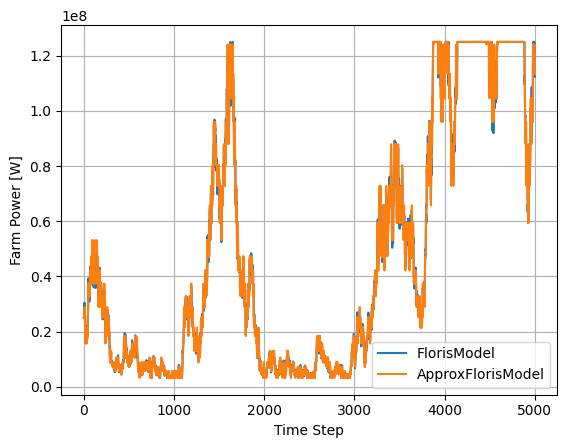
# Plot the power output from both models
fig, ax = plt.subplots()
ax.plot(fmodel.get_farm_power(), label="FlorisModel")
ax.plot(afmodel.get_farm_power(), label="ApproxFlorisModel")
ax.set_xlabel("Time Step")
ax.set_ylabel("Farm Power [W]")
ax.legend()
ax.grid(True)


# Compare the expected power results
print(f"Expected power from FlorisModel: {fmodel.get_expected_farm_power()/1E6:0.2f} MW")
print(f"Expected power from ApproxFlorisModel: {afmodel.get_expected_farm_power()/1E6:0.2f} MW")

plt.show()
import warnings
warnings.filterwarnings('ignore')

