FLORIS Models

This notebook provides information on the provided FlorisModels. Introductory Concepts introduced FlorisModel as the base class for all models in the FLORIS package. This notebook introduces the ParFlorisModel, UncertainFlorisModel, and ApproxFlorisModel classes, which are subclasses or compositions of FlorisModel.

Parallelized FLORIS Model

The ParFlorisModel class is a subclass of FlorisModel that parallelizes the FLORIS calculations. This class is designed to have an interface that is the same as FlorisModel, but the calculations are parallelized.

Instantiation

The ParFlorisModel class can be instantiated in the same way as the FlorisModel class, or else it can be instantiated by passing a FlorisModel object to the constructor.

from floris import FlorisModel, ParFlorisModel, TimeSeries
import numpy as np
import matplotlib.pyplot as plt

fmodel = FlorisModel("gch.yaml")

# Instantiation using yaml input file
pfmodel = ParFlorisModel("gch.yaml")

# Instantiation using fmodel
pfmodel = ParFlorisModel(fmodel)

Parameters

The ParFlorisModel class has additional parameters the define the parallelization. These parameters are:

interface: The parallelization interface to use. Options are "multiprocessing", "pathos", and "concurrent", with possible future support for "mpi4py"

max_workers: The maximum number of workers to use. Defaults to -1, which then takes the number of CPUs available.

n_wind_condition_splits: The number of wind conditions to split the simulation over. Defaults to the same as max_workers.

return_turbine_powers_only: Whether to return only the turbine powers.

print_timings (bool): Print the computation time to the console. Defaults to False.

# Alternative parameters
pfmodel = ParFlorisModel(fmodel, max_workers=2)

Usage

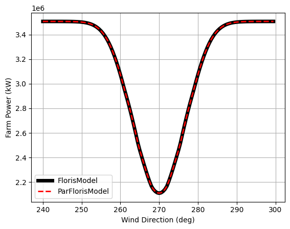
The ParFlorisModel class can be used in the same way as the FlorisModel class. The only difference is that the calculations are parallelized.

# Set to a two turbine layout
layout_x = [0, 500]
layout_y = [0, 0]
fmodel.set(layout_x=layout_x, layout_y=layout_y)
pfmodel.set(layout_x=layout_x, layout_y=layout_y)

wind_directions = np.arange(240, 300, 0.5)
time_series = TimeSeries(
    wind_directions=wind_directions, wind_speeds=8.0, turbulence_intensities=0.06
)
fmodel.set(wind_data=time_series)
pfmodel.set(wind_data=time_series)

fmodel.run()
pfmodel.run()

farm_power = fmodel.get_farm_power()
pfarm_power = pfmodel.get_farm_power()

# Show the results are the same
fig, ax = plt.subplots()
ax.plot(wind_directions, farm_power, label="FlorisModel", color='k', lw=5)
ax.plot(wind_directions, pfarm_power, label="ParFlorisModel", color='r', ls='--', lw=2)
ax.set_xlabel("Wind Direction (deg)")
ax.set_ylabel("Farm Power (kW)")
ax.legend()
ax.grid()

UncertainFlorisModel

The UncertainFlorisModel class is a composition of FlorisModel that adds uncertainty to the input conditions. Its interface is meant to made similar to FlorisModel, but with the addition of uncertainty in wind direction.

Instantiation

The UncertainFlorisModel class can be instantiated in the same way as the FlorisModel class, or else it can be instantiated by passing a FlorisModel object to the constructor. Alternatively a ParFlorisModel object can be passed to the constructor which ensures the underlying calculations are parallelized according to the ParFlorisModel parameters.

from floris import UncertainFlorisModel

# Instantiation options
ufmodel = UncertainFlorisModel("gch.yaml") # Using input yaml
ufmodel = UncertainFlorisModel(fmodel) # Using a FlorisModel object
ufmodel = UncertainFlorisModel(pfmodel) # Using a ParFlorisModel object

Parameters

To include uncertainty into the wind direction, the UncertainFlorisModel class, for each findex run, the result for a wind direction is provided by performing a Gaussian blend over results from multiple wind directions nearby wind directions. To reduce the total number of calculations required, a resolution of wind direction, wind speed, turbulence intensity and control inputs are specified and repeated calculations are only calculated once. See the class API for complete details but some key parameters are:

wd_resolution, ws_resolution, ti_resolution, yaw_resolution, and power_setpoint_resolution: Define the granularity of calculations for wind direction, wind speed, turbulence intensity, yaw angle, and power setpoints, respectively.

wd_std: The standard deviation of wind direction, used in the Gaussian blending.

wd_sample_points: Specific wind direction points to sample for expanded conditions.

# Define the uncertainty to have a wd_std of 5 degrees and blend over 10 degrees
ufmodel = UncertainFlorisModel(fmodel, wd_std=5, wd_sample_points=[-5, -4, -3, -2, -1, 0, 1, 2,3, 4, 5], wd_resolution=0.5)

Usage

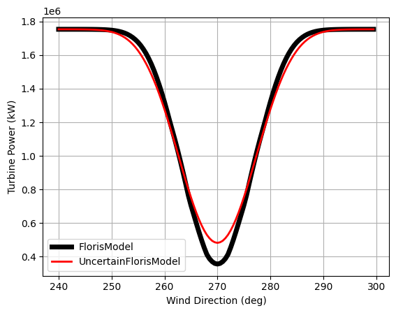
Usage of UncertainFlorisModel is similar to FlorisModel however the results will now include the effects of Gaussian blending

ufmodel.set(wind_data=time_series, layout_x=layout_x, layout_y=layout_y)
ufmodel.run()

# Get the power of the downstream turbine
f_power = fmodel.get_turbine_powers()[:,1]
uf_power = ufmodel.get_turbine_powers()[:,1]

# Plot the two powers
fig, ax = plt.subplots()
ax.plot(wind_directions, f_power, label="FlorisModel", color='k', lw=5)
ax.plot(wind_directions, uf_power, label="UncertainFlorisModel", color='r', lw=2)
ax.set_xlabel("Wind Direction (deg)")
ax.set_ylabel("Turbine Power (kW)")
ax.legend()
ax.grid()

ApproxFlorisModel

The ApproxFlorisModel overloads the UncertainFlorisModel with the special case that the wd_sample_points = [0]. This is a special case where no uncertainty is added but the resolution of the values wind direction, wind speed etc are still reduced by the specified resolution. This allows for cases to be reused and a faster approximate result computed

Instantiation

ApproxFlorisModel can be instantiated in the same way as the UncertainFlorisModel class

from floris import ApproxFlorisModel

# Instantiation options
amodel = ApproxFlorisModel("gch.yaml") # Using input yaml
amodel = ApproxFlorisModel(fmodel) # Using a FlorisModel object
amodel = ApproxFlorisModel(pfmodel) # Using a ParFlorisModel object

Usage

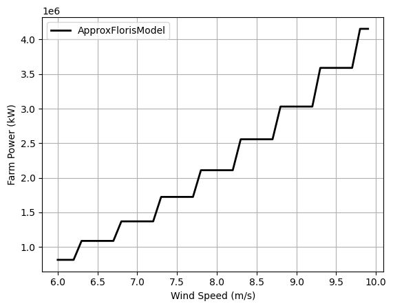
ApproxFlorisModel is used in the same way as UncertainFlorisModel but with the special case that the wd_sample_points = [0]. This means that while the resolution of the values wind_direction, wind_speeds etc are still reduced by the specified resolution, no uncertainty is added. It is intended for quickly processing large sets of inflow conditions (e.g., when reproducing SCADA records), when approximate solutions are sufficient.

# Instantiate with a wind speed resolution of 0.5 m/s and a wind direction resolution of 1 degree
amodel = ApproxFlorisModel(fmodel, ws_resolution=0.5, wd_resolution=1.0) 

# Show approximation for a time series including smaller increments of wind speed
wind_speeds = np.arange(6, 10, 0.1)
time_series = TimeSeries(
    wind_directions = 270.0,
    wind_speeds=wind_speeds,
    turbulence_intensities=0.06
)
amodel.set(wind_data=time_series)

print(f"amodel has an n_findex of {amodel.n_findex}, ",
      f"however, the number of unique cases to run at this resolution is {amodel.n_unique}.")

amodel.run()
farm_power = amodel.get_farm_power()

amodel has an n_findex of 40,  however, the number of unique cases to run at this resolution is 9.

# Show the farm power over wind speeds
fig, ax = plt.subplots()
ax.plot(wind_speeds, farm_power, label="ApproxFlorisModel", color='k', lw=2)
ax.legend()
ax.set_xlabel("Wind Speed (m/s)")
ax.set_ylabel("Farm Power (kW)")
ax.grid()