Example of using the simple-derating control model in FLORIS.

"""Example of using the simple-derating control model in FLORIS.

This example demonstrates how to use the simple-derating control model in FLORIS.
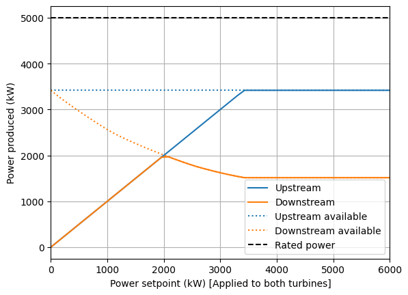
The simple-derating control model allows the user to specify a power setpoint for each turbine
in the farm. The power setpoint is used to derate the turbine power output to be at most the
power setpoint.

In this example:

1. A simple two-turbine layout is created.
2. The wind conditions are set to be constant.
3. The power setpoint is varied, and set the same for each turbine
4. The power produced by each turbine is computed and plotted
"""

import matplotlib.pyplot as plt
import numpy as np

from floris import FlorisModel


fmodel = FlorisModel("../inputs/gch.yaml")

# Change to the simple-derating model turbine
# (Note this could also be done with the mixed model)
fmodel.set_operation_model("simple-derating")

# Convert to a simple two turbine layout with derating turbines
fmodel.set(layout_x=[0, 1000.0], layout_y=[0.0, 0.0])

# For reference, load the turbine type
turbine_type = fmodel.core.farm.turbine_definitions[0]

# Set the wind directions and speeds to be constant over n_findex = N time steps
N = 50
fmodel.set(
    wind_directions=270 * np.ones(N),
    wind_speeds=10.0 * np.ones(N),
    turbulence_intensities=0.06 * np.ones(N),
)
fmodel.run()
turbine_powers_orig = fmodel.get_turbine_powers()

# Add derating level to both turbines
power_setpoints = np.tile(np.linspace(1, 6e6, N), 2).reshape(2, N).T
fmodel.set(power_setpoints=power_setpoints)
fmodel.run()
turbine_powers_derated = fmodel.get_turbine_powers()

# Compute available power at downstream turbine
power_setpoints_2 = np.array([np.linspace(1, 6e6, N), np.full(N, None)]).T
fmodel.set(power_setpoints=power_setpoints_2)
fmodel.run()
turbine_powers_avail_ds = fmodel.get_turbine_powers()[:, 1]

# Plot the results
fig, ax = plt.subplots(1, 1)
ax.plot(
    power_setpoints[:, 0] / 1000, turbine_powers_derated[:, 0] / 1000, color="C0", label="Upstream"
)
ax.plot(
    power_setpoints[:, 1] / 1000,
    turbine_powers_derated[:, 1] / 1000,
    color="C1",
    label="Downstream",
)
ax.plot(
    power_setpoints[:, 0] / 1000,
    turbine_powers_orig[:, 0] / 1000,
    color="C0",
    linestyle="dotted",
    label="Upstream available",
)
ax.plot(
    power_setpoints[:, 1] / 1000,
    turbine_powers_avail_ds / 1000,
    color="C1",
    linestyle="dotted",
    label="Downstream available",
)
ax.plot(
    power_setpoints[:, 1] / 1000,
    np.ones(N) * np.max(turbine_type["power_thrust_table"]["power"]),
    color="k",
    linestyle="dashed",
    label="Rated power",
)
ax.grid()
ax.legend()
ax.set_xlim([0, 6e3])
ax.set_xlabel("Power setpoint (kW) [Applied to both turbines]")
ax.set_ylabel("Power produced (kW)")


plt.show()
import warnings
warnings.filterwarnings('ignore')