Example: Heterogeneous Inflow in 2D and 3D

"""Example: Heterogeneous Inflow in 2D and 3D

This example showcases the heterogeneous inflow capabilities of FLORIS.
Heterogeneous flow can be defined in either 2- or 3-dimensions for a single
condition.

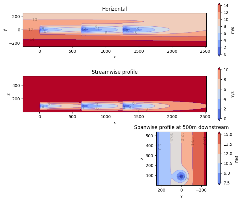
For the 2-dimensional case, it can be seen that the freestream velocity
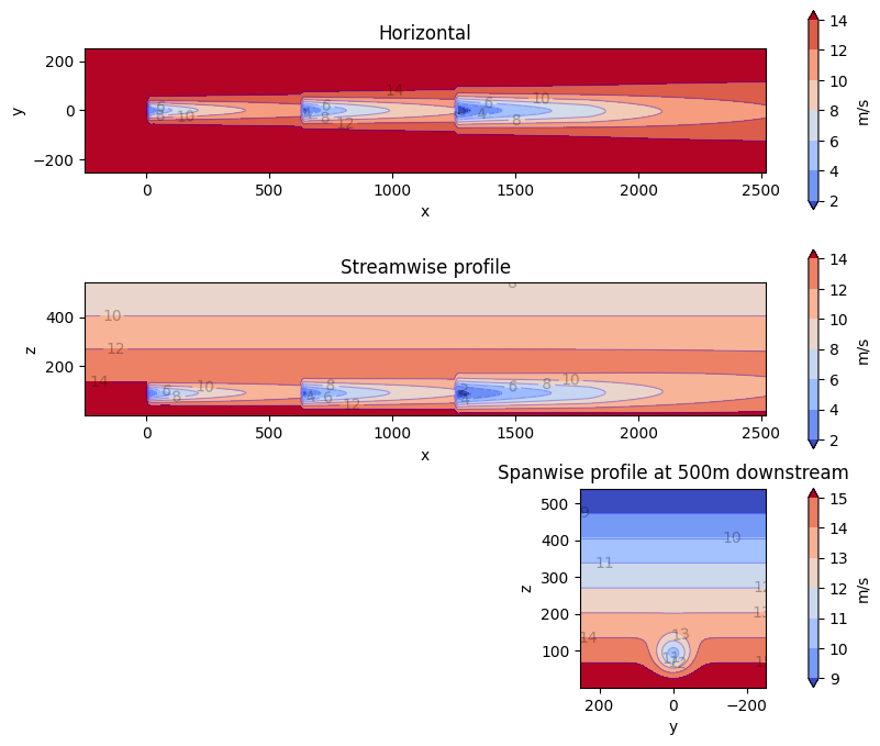
only varies in the x direction. For the 3-dimensional case, it can be
seen that the freestream velocity only varies in the z direction. This
is because of how the speed ups for each case were defined. More complex
inflow conditions can be defined.

For each case, we are plotting three slices of the resulting flow field:
1. Horizontal slice parallel to the ground and located at the hub height
2. Vertical slice parallel with the direction of the wind
3. Vertical slice parallel to to the turbine disc plane

Since the intention is for plotting, only a single condition is run and in
this case the heterogeneous_inflow_config is more convenient to use than
heterogeneous_inflow_config_by_wd. However, the latter is more convenient
when running multiple conditions.
"""


import matplotlib.pyplot as plt

from floris import FlorisModel
from floris.flow_visualization import visualize_cut_plane


# Initialize FLORIS with the given input file via FlorisModel.
# Note that the heterogeneous flow is defined in the input file. The heterogeneous_inflow_config
# dictionary is defined as below. The speed ups are multipliers of the ambient wind speed,
# and the x and y are the locations of the speed ups.
#
# heterogeneous_inflow_config = {
#     'speed_multipliers': [[2.0, 1.0, 2.0, 1.0]],
#     'x': [-300.0, -300.0, 2600.0, 2600.0],
#     'y': [ -300.0, 300.0, -300.0, 300.0],
# }


fmodel_2d = FlorisModel("../inputs/gch_heterogeneous_inflow.yaml")

# Set shear to 0.0 to highlight the heterogeneous inflow
fmodel_2d.set(wind_shear=0.0)

# Using the FlorisModel functions for generating plots, run FLORIS
# and extract 2D planes of data.
horizontal_plane_2d = fmodel_2d.calculate_horizontal_plane(
    x_resolution=200, y_resolution=100, height=90.0
)
y_plane_2d = fmodel_2d.calculate_y_plane(x_resolution=200, z_resolution=100, crossstream_dist=0.0)
cross_plane_2d = fmodel_2d.calculate_cross_plane(
    y_resolution=100, z_resolution=100, downstream_dist=500.0
)

# Create the plots
fig, ax_list = plt.subplots(3, 1, figsize=(10, 8))
ax_list = ax_list.flatten()
visualize_cut_plane(
    horizontal_plane_2d, ax=ax_list[0], title="Horizontal", color_bar=True, label_contours=True
)
ax_list[0].set_xlabel("x")
ax_list[0].set_ylabel("y")
visualize_cut_plane(
    y_plane_2d, ax=ax_list[1], title="Streamwise profile", color_bar=True, label_contours=True
)
ax_list[1].set_xlabel("x")
ax_list[1].set_ylabel("z")
visualize_cut_plane(
    cross_plane_2d,
    ax=ax_list[2],
    title="Spanwise profile at 500m downstream",
    color_bar=True,
    label_contours=True,
)
ax_list[2].set_xlabel("y")
ax_list[2].set_ylabel("z")


# Define the speed ups of the heterogeneous inflow, and their locations.
# For the 3-dimensional case, this requires x, y, and z locations.
# The speed ups are multipliers of the ambient wind speed.
speed_multipliers = [[1.0, 1.0, 2.0, 2.0, 1.0, 1.0, 2.0, 2.0]]
x_locs = [-300.0, -300.0, -300.0, -300.0, 2600.0, 2600.0, 2600.0, 2600.0]
y_locs = [-300.0, 300.0, -300.0, 300.0, -300.0, 300.0, -300.0, 300.0]
z_locs = [540.0, 540.0, 0.0, 0.0, 540.0, 540.0, 0.0, 0.0]

# Create the configuration dictionary to be used for the heterogeneous inflow.
heterogeneous_inflow_config = {
    "speed_multipliers": speed_multipliers,
    "x": x_locs,
    "y": y_locs,
    "z": z_locs,
}

# Initialize FLORIS with the given input file.
# Note that we initialize FLORIS with a homogenous flow input file, but
# then configure the heterogeneous inflow via the reinitialize method.
fmodel_3d = FlorisModel("../inputs/gch.yaml")
fmodel_3d.set(heterogeneous_inflow_config=heterogeneous_inflow_config)

# Set shear to 0.0 to highlight the heterogeneous inflow
fmodel_3d.set(wind_shear=0.0)

# Using the FlorisModel functions for generating plots, run FLORIS
# and extract 2D planes of data.
horizontal_plane_3d = fmodel_3d.calculate_horizontal_plane(
    x_resolution=200, y_resolution=100, height=90.0
)
y_plane_3d = fmodel_3d.calculate_y_plane(x_resolution=200, z_resolution=100, crossstream_dist=0.0)
cross_plane_3d = fmodel_3d.calculate_cross_plane(
    y_resolution=100, z_resolution=100, downstream_dist=500.0
)

# Create the plots
fig, ax_list = plt.subplots(3, 1, figsize=(10, 8))
ax_list = ax_list.flatten()
visualize_cut_plane(
    horizontal_plane_3d, ax=ax_list[0], title="Horizontal", color_bar=True, label_contours=True
)
ax_list[0].set_xlabel("x")
ax_list[0].set_ylabel("y")
visualize_cut_plane(
    y_plane_3d, ax=ax_list[1], title="Streamwise profile", color_bar=True, label_contours=True
)
ax_list[1].set_xlabel("x")
ax_list[1].set_ylabel("z")
visualize_cut_plane(
    cross_plane_3d,
    ax=ax_list[2],
    title="Spanwise profile at 500m downstream",
    color_bar=True,
    label_contours=True,
)
ax_list[2].set_xlabel("y")
ax_list[2].set_ylabel("z")

plt.show()
import warnings
warnings.filterwarnings('ignore')