"""Example: Wind Data Comparisons
In this example, a random time series of wind speeds, wind directions, turbulence
intensities, and values is generated. Value represents the value of the power
generated at each time step or wind condition (e.g., the price of electricity). This
can then be used in later optimization methods to optimize for total value instead of
energy. This time series is then used to instantiate a TimeSeries object. The TimeSeries
object is then used to instantiate a WindRose object and WindTIRose object based on the
same data. The three objects are then each used to drive a FLORIS model of a simple
two-turbine wind farm. The annual energy production (AEP) and annual value production
(AVP) outputs are then compared and printed to the console.
"""
import matplotlib.pyplot as plt
import numpy as np
from floris import (
FlorisModel,
TimeSeries,
)
from floris.utilities import wrap_360
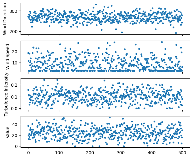
# Generate a random time series of wind speeds, wind directions, turbulence
# intensities, and values. In this case let's treat value as the dollars per MWh.
N = 500
rng = np.random.default_rng(0)
wd_array = wrap_360(270 * np.ones(N) + rng.standard_normal(N) * 20)
ws_array = np.clip(8 * np.ones(N) + rng.standard_normal(N) * 8, 3, 50)
ti_array = np.clip(0.1 * np.ones(N) + rng.standard_normal(N) * 0.05, 0, 0.25)
value_array = np.clip(25 * np.ones(N) + rng.standard_normal(N) * 10, 0, 100)
fig, axarr = plt.subplots(4, 1, sharex=True, figsize=(7, 6))
ax = axarr[0]
ax.plot(wd_array, marker=".", ls="None")
ax.set_ylabel("Wind Direction")
ax = axarr[1]
ax.plot(ws_array, marker=".", ls="None")
ax.set_ylabel("Wind Speed")
ax = axarr[2]
ax.plot(ti_array, marker=".", ls="None")
ax.set_ylabel("Turbulence Intensity")
ax = axarr[3]
ax.plot(value_array, marker=".", ls="None")
ax.set_ylabel("Value")
# Build the time series
time_series = TimeSeries(wd_array, ws_array, turbulence_intensities=ti_array, values=value_array)
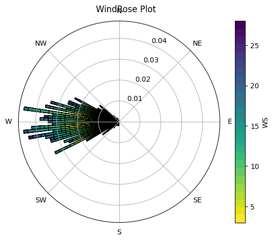
# Now build the wind rose
wind_rose = time_series.to_WindRose()
# Plot the wind rose
fig, ax = plt.subplots(subplot_kw={"polar": True})
wind_rose.plot(ax=ax, legend_kwargs={"label": "WS"})
fig.suptitle("WindRose Plot")
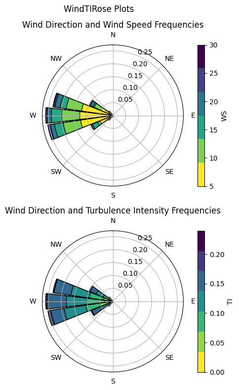
# Now build a wind rose with turbulence intensity
wind_ti_rose = time_series.to_WindTIRose()
# Plot the wind rose with TI
fig, axs = plt.subplots(2, 1, figsize=(6, 8), subplot_kw={"polar": True})
wind_ti_rose.plot(ax=axs[0], wind_rose_var="ws", legend_kwargs={"label": "WS"})
axs[0].set_title("Wind Direction and Wind Speed Frequencies")
wind_ti_rose.plot(ax=axs[1], wind_rose_var="ti", legend_kwargs={"label": "TI"})
axs[1].set_title("Wind Direction and Turbulence Intensity Frequencies")
fig.suptitle("WindTIRose Plots")
plt.tight_layout()
# Now set up a FLORIS model and initialize it using the time series and wind rose
fmodel = FlorisModel("../inputs/gch.yaml")
fmodel.set(layout_x=[0, 500.0], layout_y=[0.0, 0.0])
fmodel_time_series = fmodel.copy()
fmodel_wind_rose = fmodel.copy()
fmodel_wind_ti_rose = fmodel.copy()
fmodel_time_series.set(wind_data=time_series)
fmodel_wind_rose.set(wind_data=wind_rose)
fmodel_wind_ti_rose.set(wind_data=wind_ti_rose)
fmodel_time_series.run()
fmodel_wind_rose.run()
fmodel_wind_ti_rose.run()
# Now, compute AEP using the FLORIS models initialized with the three types of
# WindData objects. The AEP values are very similar but not exactly the same
# because of the effects of binning in the wind roses.
time_series_aep = fmodel_time_series.get_farm_AEP()
wind_rose_aep = fmodel_wind_rose.get_farm_AEP()
wind_ti_rose_aep = fmodel_wind_ti_rose.get_farm_AEP()
print(f"AEP from TimeSeries {time_series_aep / 1e9:.2f} GWh")
print(f"AEP from WindRose {wind_rose_aep / 1e9:.2f} GWh")
print(f"AEP from WindTIRose {wind_ti_rose_aep / 1e9:.2f} GWh")
# Now, compute annual value production (AVP) using the FLORIS models initialized
# with the three types of WindData objects. The AVP values are very similar but
# not exactly the same because of the effects of binning in the wind roses.
time_series_avp = fmodel_time_series.get_farm_AVP()
wind_rose_avp = fmodel_wind_rose.get_farm_AVP()
wind_ti_rose_avp = fmodel_wind_ti_rose.get_farm_AVP()
print(f"Annual Value Production (AVP) from TimeSeries {time_series_avp / 1e6:.2f} dollars")
print(f"AVP from WindRose {wind_rose_avp / 1e6:.2f} dollars")
print(f"AVP from WindTIRose {wind_ti_rose_avp / 1e6:.2f} dollars")
plt.show()
import warnings
warnings.filterwarnings('ignore')