"""Example: Optimize Layout
This example shows a simple layout optimization using the python module Scipy, optimizing for both
annual energy production (AEP) and annual value production (AVP).
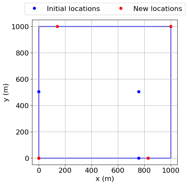
First, a 4 turbine array is optimized such that the layout of the turbine produces the
highest AEP based on the given wind resource. The turbines
are constrained to a square boundary and a random wind resource is supplied. The results
of the optimization show that the turbines are pushed to near the outer corners of the boundary,
which, given the generally uniform wind rose, makes sense in order to maximize the energy
production by minimizing wake interactions.
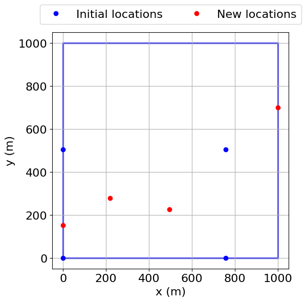
Next, with the same boundary, the same 4 turbine array is optimized to maximize AVP instead of AEP,
using the value table defined in the WindRose object, where value represents the value of the
energy produced for a given wind condition (e.g., the price of electricity). In this example, value
is defined to be significantly higher for northerly and southerly wind directions, and zero when
the wind is from the east or west. Because the value is much higher when the wind is from the north
or south, the turbines are spaced apart roughly evenly in the x direction while being relatively
close in the y direction to avoid wake interactions for northerly and southerly winds. Although the
layout results in large wake losses when the wind is from the east or west, these losses do not
significantly impact the objective function because of the low value for those wind directions.
"""
import os
import matplotlib.pyplot as plt
import numpy as np
from floris import FlorisModel, WindRose
from floris.optimization.layout_optimization.layout_optimization_scipy import (
LayoutOptimizationScipy,
)
# Define scipy optimization parameters
opt_options = {
"maxiter": 20,
"disp": True,
"iprint": 2,
"ftol": 1e-12,
"eps": 0.05,
}
# Initialize the FLORIS interface fi
fmodel = FlorisModel('../inputs/gch.yaml')
# Setup 72 wind directions with a 1 wind speed and frequency distribution
wind_directions = np.arange(0, 360.0, 5.0)
wind_speeds = np.array([8.0])
# Shape random frequency distribution to match number of wind directions and wind speeds
freq_table = np.zeros((len(wind_directions), len(wind_speeds)))
np.random.seed(1)
freq_table[:,0] = (np.abs(np.sort(np.random.randn(len(wind_directions)))))
freq_table = freq_table / freq_table.sum()
# Define the value table such that the value of the energy produced is
# significantly higher when the wind direction is close to the north or
# south, and zero when the wind is from the east or west. Here, value is
# given a mean value of 25 USD/MWh.
value_table = (0.5 + 0.5*np.cos(2*np.radians(wind_directions)))**10
value_table = 25*value_table/np.mean(value_table)
value_table = value_table.reshape((len(wind_directions),1))
# Establish a WindRose object
wind_rose = WindRose(
wind_directions=wind_directions,
wind_speeds=wind_speeds,
freq_table=freq_table,
ti_table=0.06,
value_table=value_table
)
fmodel.set(wind_data=wind_rose)
# The boundaries for the turbines, specified as vertices
boundaries = [(0.0, 0.0), (0.0, 1000.0), (1000.0, 1000.0), (1000.0, 0.0), (0.0, 0.0)]
# Set turbine locations to 4 turbines in a rectangle
D = 126.0 # rotor diameter for the NREL 5MW
layout_x = [0, 0, 6 * D, 6 * D]
layout_y = [0, 4 * D, 0, 4 * D]
fmodel.set(layout_x=layout_x, layout_y=layout_y)
# Setup the optimization problem to maximize AEP instead of value
layout_opt = LayoutOptimizationScipy(fmodel, boundaries, optOptions=opt_options)
# Run the optimization
sol = layout_opt.optimize()
# Get the resulting improvement in AEP
print('... calculating improvement in AEP')
fmodel.run()
base_aep = fmodel.get_farm_AEP() / 1e6
fmodel.set(layout_x=sol[0], layout_y=sol[1])
fmodel.run()
opt_aep = fmodel.get_farm_AEP() / 1e6
percent_gain = 100 * (opt_aep - base_aep) / base_aep
# Print and plot the results
print(f'Optimal layout: {sol}')
print(
f'Optimal layout improves AEP by {percent_gain:.1f}% '
f'from {base_aep:.1f} MWh to {opt_aep:.1f} MWh'
)
layout_opt.plot_layout_opt_results()
# reset to the original layout
fmodel.set(layout_x=layout_x, layout_y=layout_y)
# Now set up the optimization problem to maximize annual value production (AVP)
# using the value table provided in the WindRose object.
layout_opt = LayoutOptimizationScipy(fmodel, boundaries, optOptions=opt_options, use_value=True)
# Run the optimization
sol = layout_opt.optimize()
# Get the resulting improvement in AVP
print('... calculating improvement in annual value production (AVP)')
fmodel.run()
base_avp = fmodel.get_farm_AVP() / 1e6
fmodel.set(layout_x=sol[0], layout_y=sol[1])
fmodel.run()
opt_avp = fmodel.get_farm_AVP() / 1e6
percent_gain = 100 * (opt_avp - base_avp) / base_avp
# Print and plot the results
print(f'Optimal layout: {sol}')
print(
f'Optimal layout improves AVP by {percent_gain:.1f}% '
f'from {base_avp:.1f} dollars to {opt_avp:.1f} dollars'
)
layout_opt.plot_layout_opt_results()
plt.show()
import warnings
warnings.filterwarnings('ignore')