Example: Plot velocity deficit profiles

"""Example: Plot velocity deficit profiles

This example illustrates how to plot velocity deficit profiles at several locations
downstream of a turbine. Here we use the following definition:
    velocity_deficit = (homogeneous_wind_speed - u) / homogeneous_wind_speed
        , where u is the wake velocity obtained when the incoming wind speed is the
        same at all heights and equal to `homogeneous_wind_speed`.
"""


import matplotlib.pyplot as plt
import numpy as np
from matplotlib import ticker

import floris.flow_visualization as flowviz
from floris import FlorisModel
from floris.flow_visualization import VelocityProfilesFigure
from floris.utilities import reverse_rotate_coordinates_rel_west


# The first two functions are just used to plot the coordinate system in which the
# profiles are sampled. Please go to the main function to begin the example.
def plot_coordinate_system(x_origin, y_origin, wind_direction):
    quiver_length = 1.4 * D
    plt.quiver(
        [x_origin, x_origin],
        [y_origin, y_origin],
        [quiver_length, quiver_length],
        [0, 0],
        angles=[270 - wind_direction, 360 - wind_direction],
        scale_units="x",
        scale=1,
    )
    annotate_coordinate_system(x_origin, y_origin, quiver_length)


def annotate_coordinate_system(x_origin, y_origin, quiver_length):
    x1 = np.array([quiver_length + 0.35 * D, 0.0])
    x2 = np.array([0.0, quiver_length + 0.35 * D])
    x3 = np.array([90.0, 90.0])
    x, y, _ = reverse_rotate_coordinates_rel_west(
        fmodel.wind_directions,
        x1[None, :],
        x2[None, :],
        x3[None, :],
        x_center_of_rotation=0.0,
        y_center_of_rotation=0.0,
    )
    x = np.squeeze(x, axis=0) + x_origin
    y = np.squeeze(y, axis=0) + y_origin
    plt.text(x[0], y[0], "$x_1$", bbox={"facecolor": "white"})
    plt.text(x[1], y[1], "$x_2$", bbox={"facecolor": "white"})


if __name__ == "__main__":
    D = 125.88  # Turbine diameter
    hub_height = 90.0
    homogeneous_wind_speed = 8.0

    fmodel = FlorisModel("../inputs/gch.yaml")
    fmodel.set(layout_x=[0.0], layout_y=[0.0])

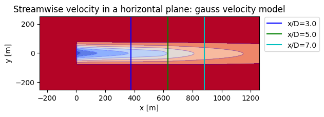
    # ------------------------------ Single-turbine layout ------------------------------
    # We first show how to sample and plot velocity deficit profiles on a single-turbine layout.
    # Lines are drawn on a horizontal plane to indicate were the velocity is sampled.
    downstream_dists = D * np.array([3, 5, 7])
    # Sample three profiles along three corresponding lines that are all parallel to the y-axis
    # (cross-stream direction). The streamwise location of each line is given in `downstream_dists`.
    profiles = fmodel.sample_velocity_deficit_profiles(
        direction="cross-stream",
        downstream_dists=downstream_dists,
        homogeneous_wind_speed=homogeneous_wind_speed,
    )

    horizontal_plane = fmodel.calculate_horizontal_plane(height=hub_height)
    fig, ax = plt.subplots(figsize=(6.4, 3))
    flowviz.visualize_cut_plane(horizontal_plane, ax)
    colors = ["b", "g", "c"]
    for i, profile in enumerate(profiles):
        # Plot profile coordinates on the horizontal plane
        ax.plot(profile["x"], profile["y"], colors[i], label=f"x/D={downstream_dists[i] / D:.1f}")
    ax.set_xlabel("x [m]")
    ax.set_ylabel("y [m]")
    ax.set_title("Streamwise velocity in a horizontal plane: gauss velocity model")
    fig.tight_layout(rect=[0, 0, 0.82, 1])
    ax.legend(bbox_to_anchor=[1.29, 1.04])

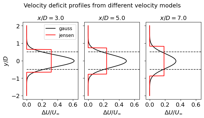
    # Initialize a VelocityProfilesFigure. The workflow is similar to a matplotlib Figure:
    # Initialize it, plot data, and then customize it further if needed.
    profiles_fig = VelocityProfilesFigure(
        downstream_dists_D=downstream_dists / D,
        layout=["cross-stream"],
        coordinate_labels=["x/D", "y/D"],
    )
    # Add profiles to the VelocityProfilesFigure. This method automatically matches the supplied
    # profiles to the initialized axes in the figure.
    profiles_fig.add_profiles(profiles, color="k")

    # Change velocity model to jensen, get the velocity deficit profiles,
    # and add them to the figure.
    floris_dict = fmodel.core.as_dict()
    floris_dict["wake"]["model_strings"]["velocity_model"] = "jensen"
    fmodel = FlorisModel(floris_dict)
    profiles = fmodel.sample_velocity_deficit_profiles(
        direction="cross-stream",
        downstream_dists=downstream_dists,
        homogeneous_wind_speed=homogeneous_wind_speed,
        resolution=400,
    )
    profiles_fig.add_profiles(profiles, color="r")

    # The dashed reference lines show the extent of the rotor
    profiles_fig.add_ref_lines_x2([-0.5, 0.5])
    for ax in profiles_fig.axs[0]:
        ax.xaxis.set_major_locator(ticker.MultipleLocator(0.2))

    profiles_fig.axs[0, 0].legend(["gauss", "jensen"], fontsize=11)
    profiles_fig.fig.suptitle(
        "Velocity deficit profiles from different velocity models",
        fontsize=14,
    )

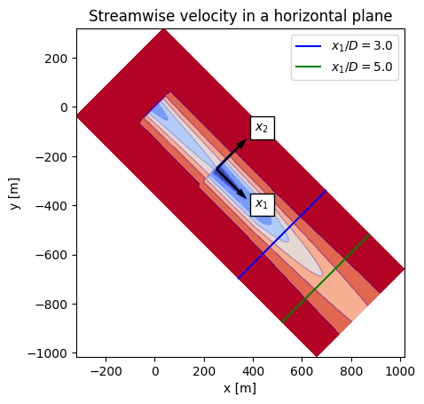
    # -------------------------------- Two-turbine layout --------------------------------
    # This is a two-turbine case where the wind direction is north-west. Velocity profiles
    # are sampled behind the second turbine. This illustrates the need for a
    # sampling-coordinate-system (x1, x2, x3) that is rotated such that x1 is always in the
    # streamwise direction. The user may define the origin of this coordinate system
    # (i.e. where to start sampling the profiles).
    wind_direction = 315.0  # Try to change this
    downstream_dists = D * np.array([3, 5])
    floris_dict = fmodel.core.as_dict()
    floris_dict["wake"]["model_strings"]["velocity_model"] = "gauss"
    fmodel = FlorisModel(floris_dict)
    # Let (x_t1, y_t1) be the location of the second turbine
    x_t1 = 2 * D
    y_t1 = -2 * D
    fmodel.set(wind_directions=[wind_direction], layout_x=[0.0, x_t1], layout_y=[0.0, y_t1])

    # Extract profiles at a set of downstream distances from the starting point (x_start, y_start)
    cross_profiles = fmodel.sample_velocity_deficit_profiles(
        direction="cross-stream",
        downstream_dists=downstream_dists,
        homogeneous_wind_speed=homogeneous_wind_speed,
        x_start=x_t1,
        y_start=y_t1,
    )

    horizontal_plane = fmodel.calculate_horizontal_plane(
        height=hub_height, x_bounds=[-2 * D, 9 * D]
    )
    ax = flowviz.visualize_cut_plane(horizontal_plane)
    colors = ["b", "g", "c"]
    for i, profile in enumerate(cross_profiles):
        ax.plot(
            profile["x"],
            profile["y"],
            colors[i],
            label=f"$x_1/D={downstream_dists[i] / D:.1f}$",
        )
    ax.set_xlabel("x [m]")
    ax.set_ylabel("y [m]")
    ax.set_title("Streamwise velocity in a horizontal plane")
    ax.legend()
    plot_coordinate_system(x_origin=x_t1, y_origin=y_t1, wind_direction=wind_direction)

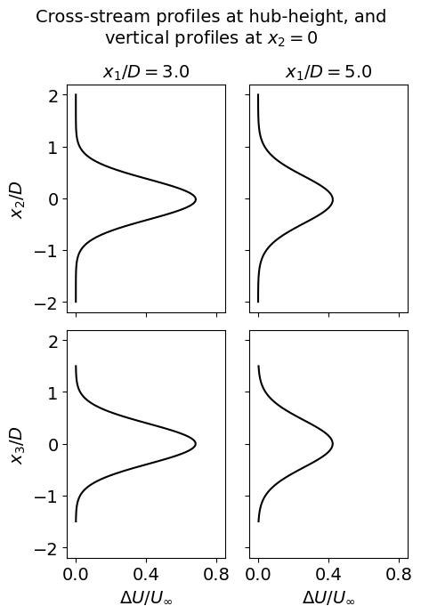
    # Sample velocity deficit profiles in the vertical direction at the same downstream
    # locations as before. We stay directly downstream of the turbine (i.e. x2 = 0). These
    # profiles are almost identical to the cross-stream profiles. However, we now explicitly
    # set the profile range. The default range is [-2 * D, 2 * D].
    vertical_profiles = fmodel.sample_velocity_deficit_profiles(
        direction="vertical",
        profile_range=[-1.5 * D, 1.5 * D],
        downstream_dists=downstream_dists,
        homogeneous_wind_speed=homogeneous_wind_speed,
        x_start=x_t1,
        y_start=y_t1,
    )

    profiles_fig = VelocityProfilesFigure(
        downstream_dists_D=downstream_dists / D,
        layout=["cross-stream", "vertical"],
    )
    profiles_fig.add_profiles(cross_profiles + vertical_profiles, color="k")

    profiles_fig.set_xlim([-0.05, 0.85])
    profiles_fig.axs[1, 0].set_ylim([-2.2, 2.2])
    for ax in profiles_fig.axs[0]:
        ax.xaxis.set_major_locator(ticker.MultipleLocator(0.4))

    profiles_fig.fig.suptitle(
        "Cross-stream profiles at hub-height, and\nvertical profiles at $x_2 = 0$",
        fontsize=14,
    )

    plt.show()
import warnings
warnings.filterwarnings('ignore')