"""Example: Compare TurbOPark model implementations
This example demonstrates a new implementation of the TurbOPark model that is
more faithful to the original description provided by Pedersen et al and uses
the sequential_solver, and compares it to the existing implementation in
Floris.
"""
import matplotlib.pyplot as plt
import numpy as np
import pandas as pd
import floris.flow_visualization as flowviz
from floris import FlorisModel, TimeSeries
from floris.turbine_library import build_cosine_loss_turbine_dict
# Note: "new" is used to refer to the new implementation of TurbOPark, which is
# more faithful to the description provided by Pedersen et al. (2022). "orig"
# is used to refer to the existing TurbOPark implementation in Floris (which
# was based on Ørsted's Matlab code, originally from Nygaard et al. (2020).
### Build a constant CT turbine model for use in comparisons (not realistic)
const_CT_turb = build_cosine_loss_turbine_dict(
turbine_data_dict={
"wind_speed":[0.0, 30.0],
"power":[0.0, 1.0], # Not realistic but won't be used here
"thrust_coefficient":[0.75, 0.75]
},
turbine_name="ConstantCT",
rotor_diameter=120.0,
hub_height=100.0,
ref_tilt=0.0,
)
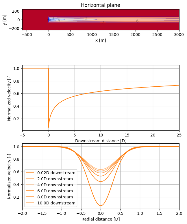
### Start by visualizing a single turbine in and its wake with the new model
# Load the new TurboPark implementation and switch to constant CT turbine
fmodel_new = FlorisModel("../inputs/turboparkgauss_cubature.yaml")
fmodel_new.set(
turbine_type=[const_CT_turb],
reference_wind_height=fmodel_new.reference_wind_height
)
fmodel_new.run()
u0 = fmodel_new.wind_speeds[0]
col_orig = "C0"
col_new = "C1"
# Get plane of points for visualization
rotor_diameter = 120.0
x_resolution=1501
y_resolution=201
z_resolution=100
x_bounds = [-5*rotor_diameter, 25*rotor_diameter]
horizontal_plane = fmodel_new.calculate_horizontal_plane(
x_resolution=x_resolution,
y_resolution=y_resolution,
height=100.0,
x_bounds=x_bounds
)
# Visualize the flows with a horizontal slice
fig, ax = plt.subplots(3,1)
fig.set_size_inches(7, 10)
flowviz.visualize_cut_plane(
horizontal_plane,
ax=ax[0],
label_contours=True,
title="Horizontal plane"
)
ax[0].set_xlabel("x [m]")
ax[0].set_ylabel("y [m]")
# Get points and velocities, normalized by rotor diameter and freestream velocity
x_locs_norm = horizontal_plane.df.x1[:x_resolution]/rotor_diameter
y_locs_norm = horizontal_plane.df.x2[::x_resolution]/rotor_diameter
u_norm = horizontal_plane.df.u[150100:151601]/u0
# Plot downstream velocities
ax[1].plot(x_locs_norm, u_norm, color=col_new)
ax[1].set_xlabel("Downstream distance [D]")
ax[1].set_ylabel("Normalized velocity [-]")
ax[1].grid()
ax[1].set_xlim([x/rotor_diameter for x in x_bounds])
# Plot axial velocities at various downstream distances
for loc in np.append(251, np.linspace(350,750,5)): #range(200,1200,200):
u_norm = horizontal_plane.df.u[int(loc)::x_resolution]/u0
alpha = 1.0 - (loc-250)/1000
ax[2].plot(y_locs_norm, u_norm, label=str((loc-250)/50)+"D downstream", alpha=alpha, c=col_new)
ax[2].legend()
ax[2].set_xlabel("Radial distance [D]")
ax[2].set_ylabel("Normalized velocity [-]")
ax[2].grid()
ax[2].set_xlim([-2, 2])
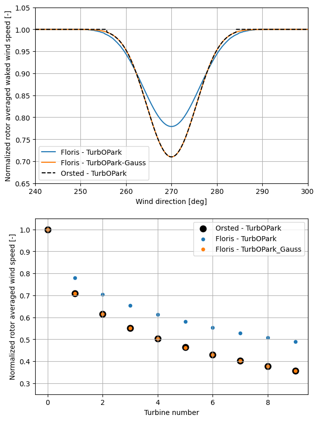
### Look at the wake profile at a single downstream distance for a range of wind directions
# Load the original TurboPark implementation and switch to constant CT turbine
fmodel_orig = FlorisModel("../inputs/turbopark_cubature.yaml")
fmodel_orig.set(
turbine_type=[const_CT_turb],
reference_wind_height=fmodel_orig.reference_wind_height
)
# Set up and solve flows
wd_array = np.arange(225,315,0.1)
wind_data_wd_sweep = TimeSeries(
wind_speeds=8.0,
wind_directions=wd_array,
turbulence_intensities=0.06
)
fmodel_orig.set(
layout_x = [0.0, 600.0],
layout_y = [0.0, 0.0],
wind_data=wind_data_wd_sweep
)
fmodel_orig.run()
# Extract output velocities at downstream turbine
orig_vels_ds = fmodel_orig.turbine_average_velocities[:,1]
u0 = fmodel_orig.wind_speeds[0] # Get freestream wind speed for normalization
# Set up and solve flows; extract velocities at downstream turbine
fmodel_new.set(
layout_x = [0.0, 600.0],
layout_y = [0.0, 0.0],
wind_data=wind_data_wd_sweep
)
fmodel_new.run()
new_vels_ds = fmodel_new.turbine_average_velocities[:,1]
# Load comparison data (generated by running Ørsted's Matlab code
# https://github.com/OrstedRD/TurbOPark)
df_twinpark = pd.read_csv("comparison_data/WindDirection_Sweep_Orsted.csv")
# Plot the data and compare
fig, ax = plt.subplots(2, 1)
fig.set_size_inches(7, 10)
ax[0].plot(wd_array, orig_vels_ds/u0, label="Floris - TurbOPark", c=col_orig)
ax[0].plot(wd_array, new_vels_ds/u0, label="Floris - TurbOPark-Gauss", c=col_new)
df_twinpark.plot("wd", "wws", ax=ax[0], linestyle="--", color="k", label="Orsted - TurbOPark")
ax[0].set_xlabel("Wind direction [deg]")
ax[0].set_ylabel("Normalized rotor averaged waked wind speed [-]")
ax[0].set_xlim(240,300)
ax[0].set_ylim(0.65,1.05)
ax[0].legend()
ax[0].grid()
### Now, look at velocities along a row of ten turbines aligned with the flow
layout_x = np.linspace(0.0, 5400.0, 10)
layout_y = np.zeros_like(layout_x)
turbines = range(len(layout_x))
wind_data_row = TimeSeries(
wind_speeds=np.array([8.0]),
wind_directions=270.0,
turbulence_intensities=0.06
)
fmodel_orig.set(
layout_x=layout_x,
layout_y=layout_y,
wind_data=wind_data_row
)
fmodel_new.set(
layout_x=layout_x,
layout_y=layout_y,
wind_data=wind_data_row
)
# Run and extract flow velocities at the turbines
fmodel_orig.run()
orig_vels_row = fmodel_orig.turbine_average_velocities
fmodel_new.run()
new_vels_row = fmodel_new.turbine_average_velocities
u0 = fmodel_orig.wind_speeds[0] # Get freestream wind speed for normalization
# Load comparison data
df_rowpark = pd.read_csv("comparison_data/Rowpark_Orsted.csv")
# Plot the data and compare
ax[1].scatter(
turbines, df_rowpark["wws"], s=80, marker="o", c="k", label="Orsted - TurbOPark"
)
ax[1].scatter(
turbines, orig_vels_row/u0, s=20, marker="o", c=col_orig, label="Floris - TurbOPark"
)
ax[1].scatter(
turbines, new_vels_row/u0, s=20, marker="o", c=col_new, label="Floris - TurbOPark_Gauss"
)
ax[1].set_xlabel("Turbine number")
ax[1].set_ylabel("Normalized rotor averaged wind speed [-]")
ax[1].set_ylim(0.25, 1.05)
ax[1].legend()
ax[1].grid()
plt.show()
import warnings
warnings.filterwarnings('ignore')