Introduction to Jupyter#

What is Jupyter?#

A web app for interactive Python in a browser

Jupyter offers a number of benefits for researchers in many fields, including:

Live coding: Make changes and see the effects in real-time.
Instant visualization: Charts and graphics render quickly in a browser window.
Sharable: Notebooks can be copied and sent to others, or multiple users can edit a single shared notebook.
Reproducible: Create a shareable environment with pinned Python and scientific library versions.
Customizable: Many configuration options, extensions, and libraries are available.
Not just for Python: Supports many other languages (including R, Julia, and many others.)
- See https://github.com/jupyter/jupyter/wiki/Jupyter-kernels for examples.

Example Notebook Code#

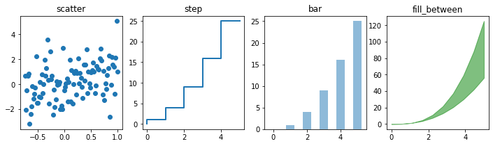
With the appropriate libraries installed into the Jupyter environment, the following code can be placed in one cell in a notebook, or split across multiple cells, and executed to produce quick graphs:

import chart_studio.plotly as py
import plotly.figure_factory as ff
import pandas as pd
import numpy as np
import matplotlib
import matplotlib.pyplot as plt
x = np.linspace(0, 5, 10)
y = x ** 2
n = np.array([0,1,2,3,4,5])
xx = np.linspace(-0.75, 1., 100)

fig, axes = plt.subplots(1, 4, figsize=(12,3))

axes[0].scatter(xx, xx + 1.25*np.random.randn(len(xx)))
#axes[0].scatter(xx, xx + 0.25*np.random.randn(len(xx)))
axes[0].set_title("scatter")

axes[1].step(n, n**2.0, lw=2)
axes[1].set_title("step")

axes[2].bar(n, n**2, align="center", width=0.5, alpha=0.5)
axes[2].set_title("bar")

axes[3].fill_between(x, x**2.5, x**3, color="green", alpha=0.5);
axes[3].set_title("fill_between");

png

Jupyter Terminology#

Jupyterhub#

This is the multi-user "backend" server. The "Hub" allows users to login, then launches the single-user Jupyter server for them. Hubs are usually installed and managed by system administrators, not Jupyter users.

NREL's "Europa" (Eagle-only) runs Jupyterhub. More on Europa later in this document.

Jupyter/Jupyter Server/Notebook server#

The single-user server/web interface. Use to create, save, or load .ipynb notebook files. This is what users generally interact with.

Jupyter Notebook#

A Notebook is an individual .pynb file. It contains your Python code and visualizations, and is sharable/downloadable.

Jupyter lab#

A "nicer" redesigned web interface for your Jupyter Server - "Notebooks 2.0". Preferred by some, and promoted as the next evolution of Notebooks. Lab has many new and different extensions, but many are also not compatible between Notebook and Lab. Lab is still under development, so is lacking some features of "classic" notebooks.

Kernel#

Kernels define the Python environments used by your notebooks. Derived from ipykernel, a predecessor project to Jupyter: you may see Jupyter kernels referred to as "ipykernels". Custom kernels require the "ipykernel" package installed in your Jupyter conda environment.

Eagle's "Europa" Jupyterhub Server#

The NREL HPC team runs a Jupyterhub server called Europa that is available for internal (NREL) Eagle users only.

Europa is connected to Eagle's Lustre storage system for access to /projects data.

A replacement for Europa on Kestrel is in the planning stage.

Europa's Advantages:#

Fast and easy access to notebooks with no setup.
Use regular Eagle credentials to log in.
Great for simple tasks, including light to moderate data processing, code debugging/testing, and light to moderate visualization using standard/basic scientific and visualization libraries.

Europa's Disadvantages:#

Limited resources: Only 48 CPU cores and 190GB RAM total.
Managed usage: Up to 8 cores/128GB RAM per user before automatic throttling will greatly slow down processing.
Must compete with other users for CPU and RAM on a single machine.
Limited list of scientific libraries and visualization tools are available, and may not be latest versions.
Custom environments are difficult to configure.
No access for external (non-NREL) users.
Not available for Kestrel (yet).

Simple Instructions to access Europa:#

Visit Europa at (https://europa.hpc.nrel.gov/) in a web browser and log in using your HPC credentials.

Europa opens a standard "notebooks" interface by default. Change the url ending from "/tree" to "/lab" in your web browser to use the Jupyter Lab interface, if preferred.

Using a Compute Node to Run Your Own Jupyter Notebooks#

Advantages:#

Custom conda environments to load preferred libraries.
Full node usage: Exclusive access to the resources of the node your job is reserved on, including up to 36 CPU cores and up to ~750GB RAM on Eagle bigmem nodes, and up to 104 CPU cores and up to ~2TB RAM on Kestrel bigmem nodes. See the system specifications page for the cluster you are working on.
No competing with other users for CPU cores and RAM, and no Arbiter2 process throttling.

Disadvantages:#

Must compete with other users for a node via the job queue.
Costs your allocation AU.

Launching Your Own Jupyter Server on an HPC System#

Both Kestrel and Eagle support running your own Jupyter Notebook server. This is highly recommended over Europa for advanced Jupyter use and heavy computational processing.

External (non-NREL) Kestrel users may follow the directions below for Kestrel, but please use kestrel.nrel.gov instead of kestrel.hpc.nrel.gov.

External (non-NREL) Eagle users will no longer be able to use Jupyter in this fashion as of February 2024. If you require Jupyter, please consider transitioning to Kestrel as soon as possible.

Using a Compute Node to run Jupyter Notebooks#

Connect to a login node and request an interactive job using the salloc command.

The examples below will start a 2-hour job. Edit the <account> to the name of your allocation, and adjust the time accordingly. Since these are interactive jobs, they will get some priority, especially if they're shorter, so only book as much time as you will be actively working on the notebook.

Before you get started, we recommend installing your own Jupyter inside of a conda environment. The default conda/anaconda3 modules contain basic Jupyter Notebook servers, but you will likely want your own Python libraries, notebook extensions, and other features. Basic directions are included later in this document.

Kestrel:#

[user@laptop:~]$ ssh kestrel.hpc.nrel.gov

[user@kl1:~]$ salloc -A <account> -t 02:00:00

Eagle:#

[user@laptop:~]$ ssh eagle.hpc.nrel.gov

[user@el1:~]$ salloc -A <account> -t 02:00:00

Starting Jupyter Inside the Job#

Once the job starts and you are allocated a compute node, load the appropriate modules, activate your Jupyter environment, and launch the Jupyter server.

Kestrel:#

[user@x1000c0s0b0n1:~]$ module load anaconda3

[user@x1000c0s0b0n1:~]$ source activate myjupenv

[user@x1000c0s0b0n1:~]$ jupyter-notebook --no-browser --ip=$(hostname -s)

Take note of the node name that your job is assigned. (x1000c0s0b0n1 in the above example.)

Also note the url that Jupyter displays when starting up, e.g. http://127.0.0.1:8888/?token=<alphabet soup>.

The <alphabet soup> is a long string of letters and numbers. This is a unique authorization token for your Jupyter session. you will need it, along with the full URL, for a later step.

Eagle:#

[user@r2i7n35:~]$ module load conda

source activate myjupenv

jupyter-notebook --no-browser --ip=$(hostname -s)

Take note of the node name that your job is assigned. (r2i7n35 in this example.)

Also note the url that Jupyter displays when starting up, e.g. http://127.0.0.1:8888/?token=<alphabet soup>.

The <alphabet soup> is a long string of letters and numbers. This is a unique authorization token for your Jupyter session. you will need it, along with the full URL, for a later step.

On Your Own Computer#

Next, open an SSH tunnel through a login node to the compute node. Log in when prompted using your regular HPC credentials, and put this terminal to the side or minimize it, but leave it open until you are done working with Jupyter for this session.

Kestrel:#

[user@laptop:~]$ ssh -N -L 8888:<nodename>:8888 username@kestrel.hpc.nrel.gov

Eagle:#

[user@laptop:~]$ ssh -N -L 8888:<nodename>:8888 username@eagle.hpc.nrel.gov

Open a Web Browser#

Copy the full url and token from Jupyter startup into your web browser. For example:

http://127.0.0.1:8888/?token=<alphabet soup>

Using a Compute Node - The Easy Way#

Scripted assistance with launching a Jupyter session on Eagle or Kestrel is available.

Internal NREL Users Only: pyeagle#

The pyeagle package is available for internal users to handle launching and monitoring a jupyter server on a compute node. This package is maintained by an NREL HPC user group, and provides utilities for working on Eagle and Kestrel.

Auto-launching on Eagle With an sbatch Script#

These scripts are designed for Eagle and may not yet be adapted for Kestrel, but may be downloaded and adapted manually.

Full directions included in the Jupyter repo.

Download sbatch_jupyter.sh and auto_launch_jupyter.sh

Edit sbatch_jupyter.sh to change:

--account=*yourallocation*

--time=*timelimit*

Run auto_launch_jupyter.sh and follow directions

That's it!

Data processing and visualization should be done via Europa or compute nodes.
Uses a highly shared resource (login nodes): there will be competition for CPU, RAM, and network I/O for storage. Arbiter2 software will automatically throttle moderate to heavy usage on login nodes, greatly slowing down processing.

Custom Conda Environments and Jupyter Kernels#

On Kestrel, the module 'anaconda3' is available to run the conda command and manage your environments.

As an alternative, the module 'mamba' is available instead. Mamba is a conda-compatible environment manager with very similar usage. Most conda commands in this documentation may be used with mamba instead and they may generally be considered interchangeable.

On Eagle, the module 'conda' contains the conda command. The Eagle conda module also contains mamba installed as a conda package.

Creating a Conda Environment#

To add your own packages to conda on Kestrel or Eagle:

Create an environment and install the base jupyter packages. Then activate the environment and install other libraries that you want to use, e.g. scipy, numpy, and so on.

conda create -n myjupyter -c conda-forge jupyter ipykernel

source activate myjupyter

conda install -c conda-forge scipy numpy matplotlib

Add Custom iPykernel#

A kernel is what allows Jupyter to use your customized conda environment inside Jupyter, in a notebook. Use ipykernel to build your kernel. Inside your custom conda environment, run:

python -m ipykernel install --user --name=myjupyter

If you already have a Jupyter server running, restart it to load the new kernel.

The new kernel will appear in the drop-down as an option to open a new notebook.

You can have multiple kernels, allowing you to load different conda environments for your different projects into Notebooks.

Jupyter Kernel Management#

Use the kernelspec list command inside your Jupyter conda environment to see what ipykernels you have installed:

jupyter kernelspec list

To remove an old kernel, use the kernelspec remove command:

jupyter kernelspec remove myoldjupyter

Magic Commands#

Magic commands are "meta commands" that add extra functionality to Jupyter.

Magic commands begin with % or %%.

Example Magic Commands#

* %lsmagic - list all magic commands
* %run _file.py_ - run an external python script
* %%time - placed at top of cell, prints execution time
* %who - list all defined variables in notebook

%lsmagic

Available line magics:
%alias  %alias_magic  %autoawait  %autocall  %automagic  %autosave  %bookmark  %cat  %cd  %clear  %colors  %conda  %config  %connect_info  %cp  %debug  %dhist  %dirs  %doctest_mode  %ed  %edit  %env  %gui  %hist  %history  %killbgscripts  %ldir  %less  %lf  %lk  %ll  %load  %load_ext  %loadpy  %logoff  %logon  %logstart  %logstate  %logstop  %ls  %lsmagic  %lx  %macro  %magic  %man  %matplotlib  %mkdir  %more  %mv  %notebook  %page  %pastebin  %pdb  %pdef  %pdoc  %pfile  %pinfo  %pinfo2  %pip  %popd  %pprint  %precision  %prun  %psearch  %psource  %pushd  %pwd  %pycat  %pylab  %qtconsole  %quickref  %recall  %rehashx  %reload_ext  %rep  %rerun  %reset  %reset_selective  %rm  %rmdir  %run  %save  %sc  %set_env  %store  %sx  %system  %tb  %time  %timeit  %unalias  %unload_ext  %who  %who_ls  %whos  %xdel  %xmode

Available cell magics:
%%!  %%HTML  %%SVG  %%bash  %%capture  %%debug  %%file  %%html  %%javascript  %%js  %%latex  %%markdown  %%perl  %%prun  %%pypy  %%python  %%python2  %%python3  %%ruby  %%script  %%sh  %%svg  %%sx  %%system  %%time  %%timeit  %%writefile

Automagic is ON, % prefix IS NOT needed for line magics.

Shell Commands#

You can also run shell commands inside a cell. For example:

!conda list - see the packages installed in the environment you're using

!pwd
!ls

/home/username/jup
auto_launch_jupyter.sh    Jupyter Presentation.ipynb  slurm-6445885.out
geojsondemo.ipynb         old                         sshot1.png
Interesting Graphs.ipynb  sbatch_jupyter.sh           sshot2.png
jup-logo.png              slurm