reV documentation

What is reV?

reV (the Renewable Energy Potential model) is an open-source geospatial techno-economic tool that estimates renewable energy technical potential (capacity and generation), system cost, and supply curves for solar photovoltaics (PV), concentrating solar power (CSP), geothermal, and wind energy. reV allows researchers to include exhaustive spatial representation of the built and natural environment into the generation and cost estimates that it computes.

reV is highly dynamic, allowing analysts to assess potential at varying levels of detail — from a single site up to an entire continent at temporal resolutions ranging from five minutes to hourly, spanning a single year or multiple decades. The reV model can (and has been used to) provide broad coverage across large spatial extents, including North America, South and Central Asia, the Middle East, South America, and South Africa to inform national and international-scale analyses. Still, reV is equally well-suited for regional infrastructure and deployment planning and analysis.

For a detailed description of reV capabilities and functionality, see the NREL reV technical report.

How does reV work?

reV is a set of Python classes and functions that can be executed on HPC systems using CLI commands. A full reV execution consists of one or more compute modules (each consisting of their own Python class/CLI command) strung together using a pipeline framework, or configured using batch.

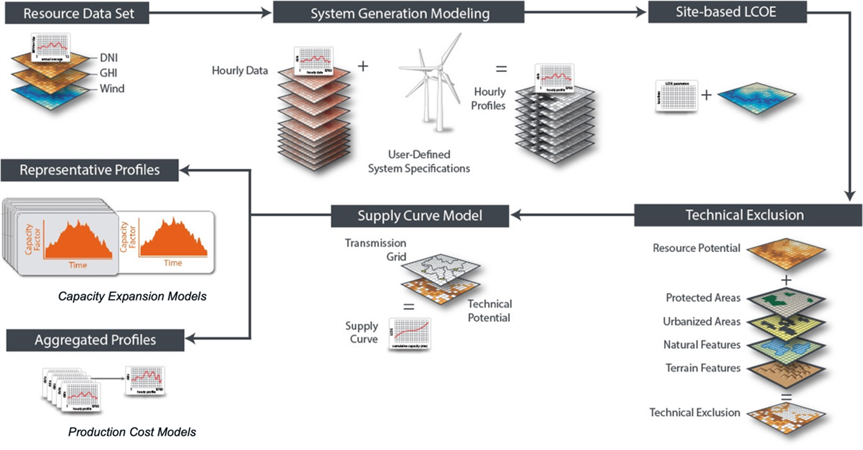
A typical reV workflow begins with input wind/solar/geothermal resource data (following the rex data format) that is passed through the generation module. This output is then collected across space and time (if executed on the HPC), before being sent off to be aggregated under user-specified land exclusion scenarios. Exclusion data is typically provided via a collection of high-resolution spatial data layers stored in an HDF5 file. This file must be readable by reV’s ExclusionLayers class. See the reVX Setbacks utility for instructions on generating setback exclusions for use in reV. Next, transmission costs are computed for each aggregated “supply-curve point” using user-provided transmission cost tables. See the reVX transmission cost calculator utility for instructions on generating transmission cost tables. Finally, the supply curves and initial generation data can be used to extract representative generation profiles for each supply curve point.

A visual summary of this process is given below:

To get up and running with reV, first head over to the installation page, then check out some of the Examples or go straight to the CLI Documentation! You can also check out the guide on running GAPs models.

Installing reV

NOTE: The installation instruction below assume that you have python installed on your machine and are using conda as your package/environment manager.

Option 1: Install from PIP (recommended for analysts):

1. Create a new environment:

   conda create --name rev python=3.9

2. Activate directory:

   conda activate rev

3. Install reV:

   1. pip install NREL-reV or

      • NOTE: If you install using conda and want to use HSDS you will also need to install h5pyd manually: pip install h5pyd

Option 2: Clone repo (recommended for developers)

1. from home dir, git clone git@github.com:NREL/reV.git

2. Create reV environment and install package

   1. Create a conda env: conda create -n rev

   2. Run the command: conda activate rev

   3. cd into the repo cloned in 1.

   4. prior to running pip below, make sure the branch is correct (install from main!)

   5. Install reV and its dependencies by running: pip install . (or pip install -e . if running a dev branch or working on the source code)

3. Check that reV was installed successfully

   1. From any directory, run the following commands. This should return the help pages for the CLI’s.

      • reV

reV command line tools

• reV

• reV template-configs

• reV batch

• reV pipeline

• reV project-points

• reV bespoke

• reV generation

• reV econ

• reV collect

• reV multiyear

• reV supply-curve-aggregation

• reV supply-curve

• reV rep-profiles

• reV hybrids

• reV nrwal

• reV qa-qc

• reV script

• reV status

• reV reset-status

Launching a run

Tips

• Only use a screen session if running the pipeline module: screen -S rev

• Full pipeline execution

reV pipeline -c "/scratch/user/rev/config_pipeline.json"

• Running simply generation or econ can just be done from the console:

reV generation -c "/scratch/user/rev/config_gen.json"

General Run times and Node configuration on Eagle

• WTK Conus: 10-20 nodes per year walltime 1-4 hours

• NSRDB Conus: 5 nodes walltime 2 hours

Eagle node requests

Recommended Citation

Please cite both the technical paper and the software with the version and DOI you used:

Maclaurin, Galen J., Nicholas W. Grue, Anthony J. Lopez, Donna M. Heimiller, Michael Rossol, Grant Buster, and Travis Williams. 2019. “The Renewable Energy Potential (reV) Model: A Geospatial Platform for Technical Potential and Supply Curve Modeling.” Golden, Colorado, United States: National Renewable Energy Laboratory. NREL/TP-6A20-73067. https://doi.org/10.2172/1563140.

Grant Buster, Michael Rossol, Paul Pinchuk, Brandon N Benton, Robert Spencer, Mike Bannister, & Travis Williams. (2023). NREL/reV: reV 0.8.0 (v0.8.0). Zenodo. https://doi.org/10.5281/zenodo.8247528