Parameter calibration for Normal and Beta distributions

This tutorial demonstrates how to conduct the calibration with and without a surrogate forward model

Running the tutorial

We assume that bird is installed within an environment called bird (see either the Installation section for developers or the Installation section for users)

You will need to install additional dependencies

conda activate bird
BIRD_DIR = `python -c "import bird; print(bird.BIRD_DIR)"`
cd ${BIRD_DIR}/../
pip install .[calibration]

The calibration tutorial is located at ${BIRD_DIR}/../tutorial_cases/calibration/normal_beta

Calibration Objective

The PDF of a Beta(alpha,beta) distribution is observed. Within the context of bioreactors, one can consider this PDF to be a measured bubble size distribution (BSD)

A separate dummy numerical model is available and predicts BSD as normal distributions N(mu, sigma). The input parameter of the numerical models are mu and sigma. The objective of the modeler is to find mu and sigma such that the predicted BSD matches the observed BSD

We assume that the numerical model is expensive and instead of using the expensive numerical model for the forward model used in the calibration, one would like to use a cheaper surrogate model. Here the surrogate model is a neural network.

Building the surrogate

The class Param_NN available in BiRD allows to create a parametric surrogate. Here, the input of the surrogate are the parameters mu and sigma, and the variable x that parameterize the PDF.

Constructing such a surrogate is not computationally useful here since the forward simulation is cheap. This is only for illustrative purposes!

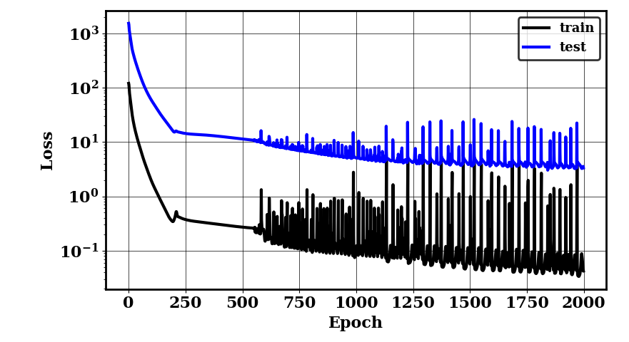
Generate dataset and train neural net surrogate with python tut_surrogate.py. The following plots should be generated. The first one shows the training and testing loss convergence. The second one shows examples of the surrogate accuracy on unseen data.

Calibration with optimized likelihood uncertainty

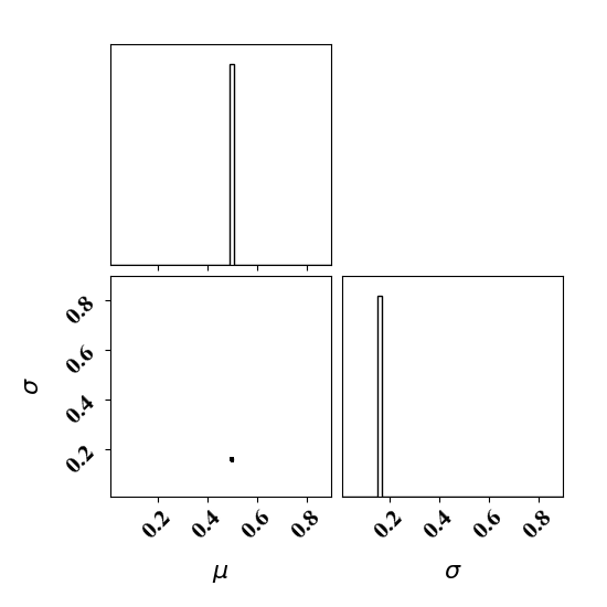
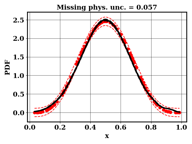
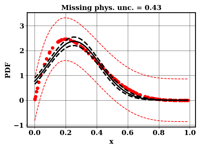
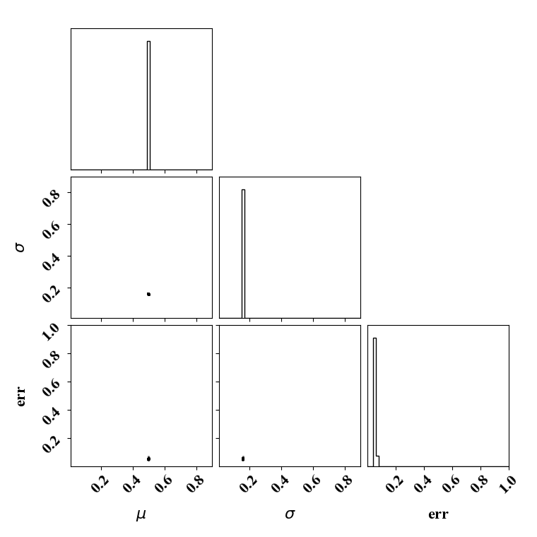
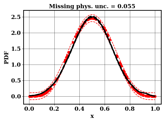
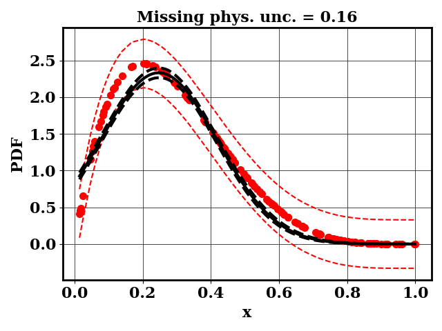
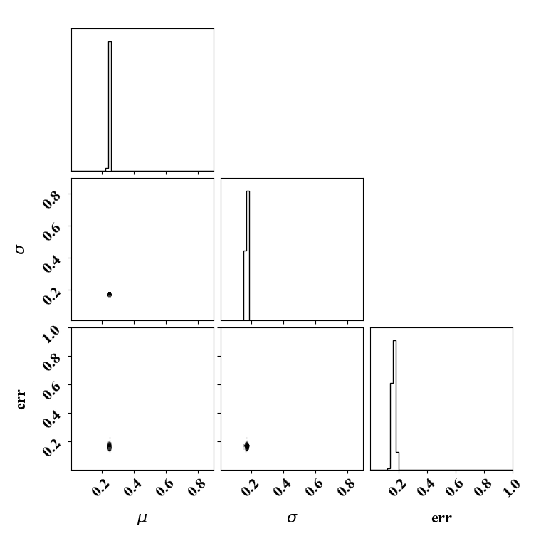
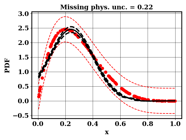
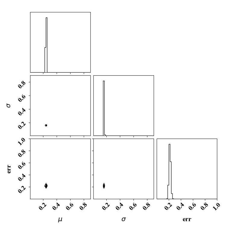
For the calibration, we can use the true function or the surrogate model. The objective PDF is assumed to be noiseless. Even though the observation is noiseless, an uncertainty is computed to account for the missing physics. The likelihood uncertainty that represents the missing physics is optimized to ensure an uncertainty band overlap

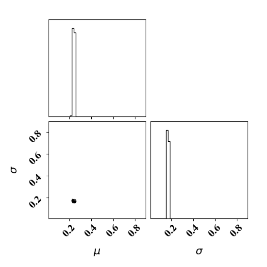
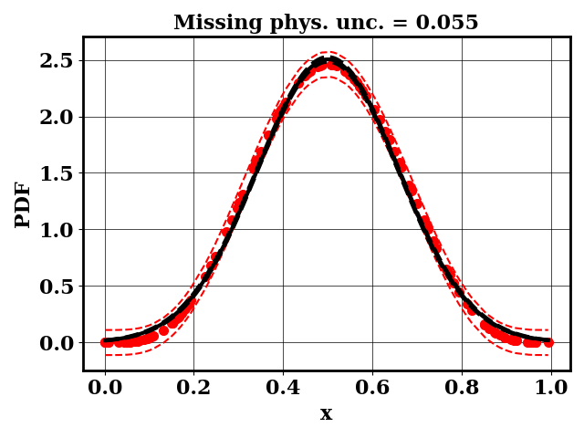
Calibrate without a surrogate for alpha=5, beta=5

python tut_calibration.py --alpha 5 --beta 5

Calibrate with a surrogate for alpha=5, beta=5

python tut_calibration.py -useNN --alpha 5 --beta 5

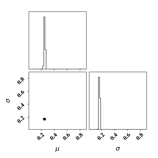
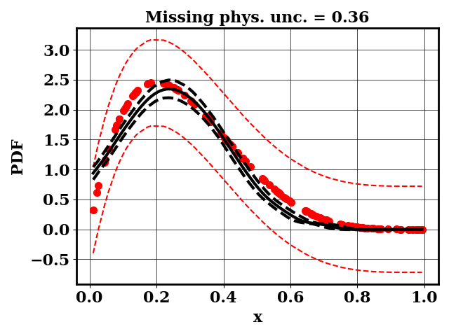
Calibrate without a surrogate for alpha=2, beta=5

python tut_calibration.py --alpha 2 --beta 5

Calibrate with a surrogate for alpha=2, beta=5

python tut_calibration.py -useNN --alpha 2 --beta 5

Clearly, the amount of missing physics vary depending on the observations.

Using surrogate gives similar predictions as when not using a surrogate. But the surrogate was constructed with 200 forward simulations. In the case where forward simulations are expensive, the surrogate modeling approach is significantly faster.

Calibration with calibrated likelihood uncertainty

The same suite can be done by calibrating the likelihood uncertainty in lieu of optimizing it (with a bissection search). This has the advantage of rapid calibration since only one calibration is needed. Here the uncertainty minimizes the negative log likelihood.

Calibrate without a surrogate for alpha=5, beta=5

python tut_calibration.py --alpha 5 --beta 5 -cal_err

Calibrate with a surrogate for alpha=5, beta=5

python tut_calibration.py -useNN --alpha 5 --beta 5 -cal_err

Calibrate without a surrogate for alpha=2, beta=5

python tut_calibration.py --alpha 2 --beta 5 -cal_err

Calibrate with a surrogate for alpha=2, beta=5

python tut_calibration.py -useNN --alpha 2 --beta 5 -cal_err