Bubble column
This tutorial demonstrates how to run a basic bubble column reactor case. The tutorial assumed you have created and activated the bird environment and setup path variables as
conda activate bird
BIRD_HOME=`python -c "import bird; print(bird.BIRD_DIR)"`
BCE_CASE=${BIRD_HOME}/../tutorial_cases/bubble_column_20L
The tutorial is located under ${BCE_CASE}
This is a code-along tutorial, and the steps are shown in order of how one would go about setting up a case. The reader can execute the commands in the order shown below
To simply run the entire tutorial, do:
cd ${BCE_CASE}
bash run.sh
This test is run as part of the continuous integration
Geometry
The geometry details are described in ${BCE_CASE}/system/mesh.json and ${BCE_CASE}/system/topology.json
All the steps in this section are done by executing
python ${BIRD_HOME}/../applications/write_block_cyl_mesh.py -i system/mesh.json -t system/topology.json -o system
This command generates the appropriate blockMeshDict
Block geometry
BiRD uses a block cylindral geometry description (Block cylindrical meshing). The block description of the geometry is in ${BCE_CASE}/system/mesh.json under the Geometry key
"Geometry": {
         "Radial": {
                 "column_trans" : 275,
                 "column" : 360
         },
         "Longitudinal": {
                 "column_top" : 12000,
                 "head_space" : 9000,
                 "sparger_trans": 1000,
                 "bottom" : 0
         }
}
Those numbers describes the coordinates of the cylindrical blocks. Using the block diagram discussed in (Block cylindrical meshing), the geometry is
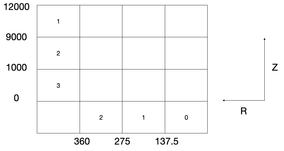
Note that the first radial number column_trans is special and results in 2 radial blocks. The first radial block is the square of the pillow-mesh where the edge is half of the first coordinate \((275/2=137.5)\). The second radial block is the outer-shell of the pillow.
By default, the coordinates of the block cylindrical geometry are in meters. In this case, the intention was to indicate millimeters instead. This will be handled during the Mesh post-treatment below.
Each one of the cylindrical blocks will be meshed because we are constructing a bubble column. So there is no need for defining one of the blocks as a wall (conversely to the example shown in Block cylindrical meshing).
The coordinate are shown in the figure above in radial coordinates but OpenFOAM only uses cartesian coordinates. The radial coordinates are transformed in \((x,y)\) cartesian coordinate for you. The longitudinal coordinate always matches the \(z\) cartesian coordinate. In our present case, we want the bubble column axis of revolution to be along the \(y\)-direction (not \(z\)). We will show in Mesh post-treatment.
Boundaries
The boundary conditions are described in ${BCE_CASE}/system/topology.json and are used to define the outlet boundary named outlet as
"Boundary": {
             "outlet":[
                        {"type": "top", "Rmin": 0, "Rmax": 0, "Lmin": 0, "Lmax": 1},
                        {"type": "top", "Rmin": 1, "Rmax": 1, "Lmin": 0, "Lmax": 1},
                        {"type": "top", "Rmin": 2, "Rmax": 2, "Lmin": 0, "Lmax": 1}
                      ]
}
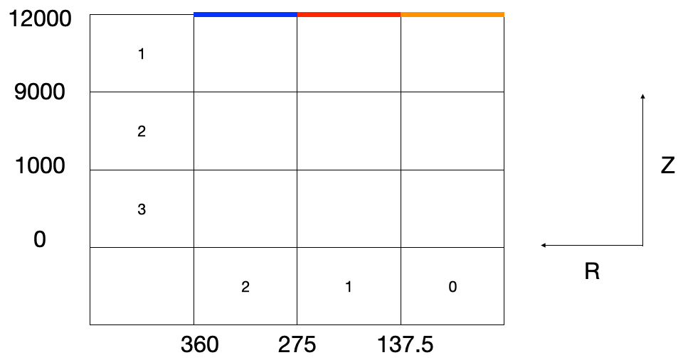
The snippet above defines outlet as the concatenation of 3 faces of cylindrical blocks. The blocks faces are defined by a pair of block: a min block and a max block. Each one of the blocks is defined by its radial index (Rmin or Rmax) and its longitudinal index (Lmin or Lmax). In the bubble column case, the three block faces that define the outlet are
The boundary between the block
(Lmin=0, Rmin=0)and the block(Lmax=1, Rmax=0)
The boundary between the block
(Lmin=0, Rmin=1)and the block(Lmax=1, Rmax=1)
The boundary between the block
(Lmin=0, Rmin=2)and the block(Lmax=1, Rmax=2)
In the graph below, the vertical block 0 and vertical block 4 are not represented. They are ghost blocks that are only used to define bounding boundaries. Likewise, the radial block 3 is not represented is another ghost block but can be used to define lateral boundaries.
To finish defining the boundaries of the bubble column, we would need to define the outer walls and the inlet. We do not define any other boundaries for now and BiRD automatically sets non-defined patches as walls. We will show how to set the inlet boundary in Inlet patch.
Mesh
The meshing is defined based on Meshing in ${BCE_CASE}/system/mesh.json
"Meshing": {
        "NRSmallest": 4,
        "NVertSmallest": 12,
The size of the radial mesh is defined using NRSmallest. It denotes the number of mesh point through the smallest radial block. Blocks at \(R=0\) (where \(R\) is the radial index of the block shown in the block diagrams above) have radial size \(137.5\), at \(R=1\) have size \(275-137.5=137.5\), and at \(R=2\) have size \(360-275=85\). The smallest radial block is at \(R=2\), so 4 mesh points will be used to mesh the radial blocks at \(R=2\).
Starting from this number, the number of points in the other radial blocks will be adjusted based on the size of the blocks, to make sure that the mesh size is constant radially. We refer to these numbers as the base mesh numbers.
The same goes for NVertSmallest in the longitudinal direction.
The mesh size can be further adjusted with the coarsening keys
"Meshing": {
 ...
        "verticalCoarsening":[
                               {"ratio": 0.5, "direction": "+", "directionRef": "-"},
                               {"ratio": 1.0, "direction": "+", "directionRef": "-"},
                               {"ratio": 1.0, "direction": "+", "directionRef": "-"}
                             ],
        "radialCoarsening":  [
                               {"ratio": 1.0, "direction": "+", "directionRef": "-"},
                               {"ratio": 1.0, "direction": "+", "directionRef": "-"}
                             ]
The ratios denote the how the base mesh numbers should be altered. By default, no alteration is done.
In the radial direction, no coarsening or refinement is done in the first two blocks. For the third one, the default setting is used (no coarsening). We recommend to avoid coarsening or refining in the radial direction at the moment: this feature is rarely used and would be prone to bugs.
In the vertical direction, no coarsening is used, except for the first block. In the first block, we reduce the number of mesh points compared to the base mesh by a factor 0.5. The mesh size is adjusted using a grading so that a smooth mesh size transition is achieved. The direction and directionRef should always be opposite signs. The directionRef denotes where to look to define a smooth transition. Here, directionRef : "-" so mesh size to achieve at the bottom of the block should match the size of the mesh in block below. This what we want, because the first vertical block is meshing the headspace, and less and less resolution is needed as \(z\) increases.
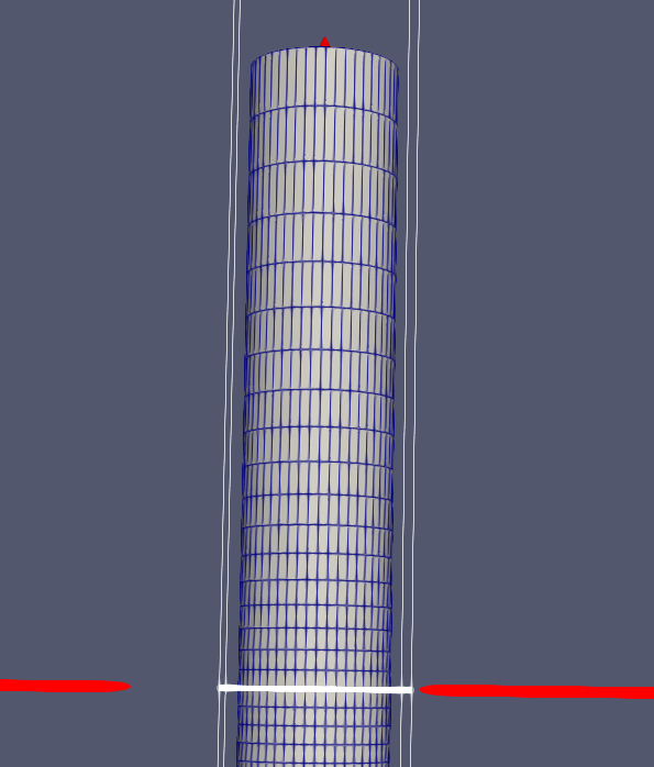
The resulting mesh looks as the picture below. The white line denotes the boundary between the first and the second vertical (also called longitudinal) block.
Mesh post-treatment
Once blockMeshDict is generated, the mesh can be constructed using the blockMesh utility of OpenFOAM
blockMesh -dict system/blockMeshDict
As mentioned earlier, one might want to define the axis of revolution of the column along the \(y\) direction, in which case, one can use
transformPoints "rotate=((0 0 1) (0 1 0))"
Finally, one might want to convert the units from \(mm\) into \(m\) , which can be done as
transformPoints "scale=(0.001 0.001 0.001)"
Inlet patch
BiRD allows for the generation of complex patches through the generation of .stl files that describe the patch geometry.
Note that we could have generated the outlet patch with another stl file (we do it in the case of the loop reactor tutorial). Here, since the outlet can be simply defined as an entire block cylindrical face, we prefer to define it that way. In the case of the inlet, only part of a block cylindrical face is the inlet, and it is more convenient to use the .stl approach.
Here, we would like to create a circular sparger centered on \((x,y,z)=(0,0,0)\), and of radius \(0.2\) m, with a normal face along the \(y\)-direction Recall that we scaled our mesh so the outer radius of the column is now \(0.360\) m, and not \(360\) m.
The inlet patch geometry is defined in ${BCE_CASE}/system/inlets_outlets.json as
"inlets": [
     {"type": "circle", "radius": 0.2, "centx": 0.0, "centy": 0.0, "centz": 0.0, "normal_dir": 1, "nelements": 50}
]
This describes exactly the properties shown above. The nelements key denote the number of triangles in the .stl.
The following command generates inlets.stl
python ${BIRD_HOME}/../applications/write_stl_patch.py -i system/inlets_outlets.json
One can visualize the inlet STL patch with Paraview and see that it indeed contains 50 triangles, and that its normal is the \(y\)-direction.
Now, the inlet must be added to the boundary in place of some of the default wall patches. This can be done using OpenFOAM utilities. By default, OpenFOAM names the patch after the .stl filename. We can change that using sed. In the end, the new patch is created as
cd ${BCE_CASE}/
surfaceToPatch -tol 1e-3 inlets.stl
export newmeshdir=$(foamListTimes -latestTime)
rm -rf constant/polyMesh/
cp -r $newmeshdir/polyMesh ./constant
rm -rf $newmeshdir
cp ${BCE_CASE}/constant/polyMesh/boundary /tmp
sed -i -e 's/inlets\.stl/inlet/g' /tmp/boundary
cat /tmp/boundary > constant/polyMesh/boundary
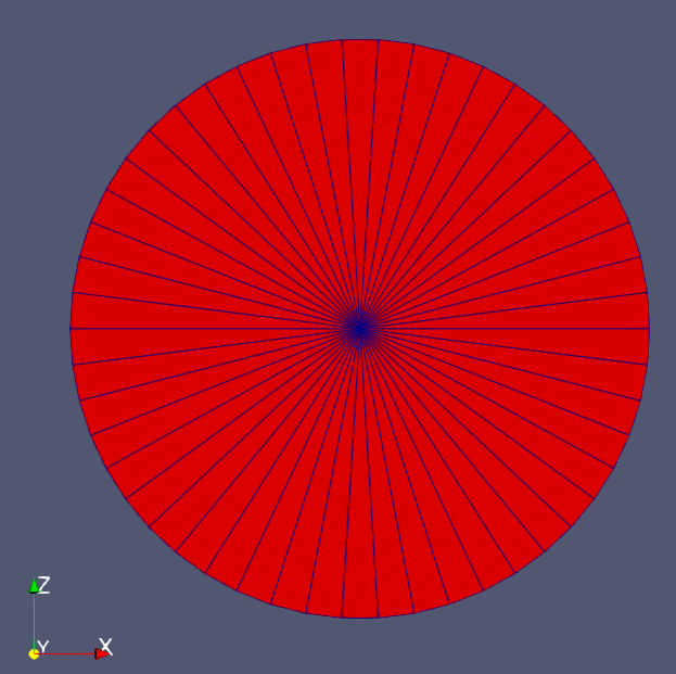
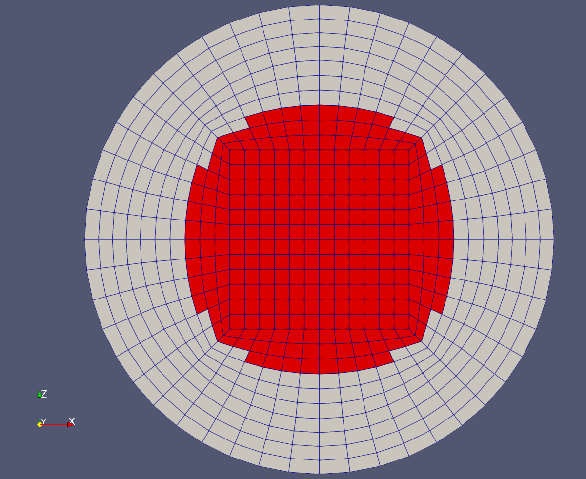
At this point, you can visualize the inlet patch in paraview. The figure below shows the inlet patch in red. One can see that the inlet patch only approximately matches the stl file. In most applications, this amount of approximation is acceptable. If it is not one could
modify the block-cylindrical mesh and make sure that the inlet exactly matches an ensemble of block cylindrical faces. Then one defines the inlet patch similarly to the way the outlet patch was constructed. This allows for a very close match to the .stl
If 1. is not possible because the sparger geometry is complex, one could use a finer mesh to allow for a close match between the stl and inlet patch.
Initial conditions
The initial conditions are defined through the ${BCE_CASE}/0/ time folder. We provide a pre-made folder ${BCE_CASE}/0.orig/. Two fields, the volume fraction of gas (alpha.gas) and liquid (alpha.liquid) are essential in a bubble column and are left for the user to define. We typically define them with the setFields utility in OpenFOAM which looks up the values defined in ${BCE_CASE}/system/setFieldsDict. The important part of the file is shown below
defaultFieldValues
(
    volScalarFieldValue alpha.gas 0.99
    volScalarFieldValue alpha.liquid 0.01
);

regions
(
    boxToCell
    {
        box (-1.0 -1.0 -1.0) (10 7 10);
        fieldValues
        (
            volScalarFieldValue alpha.gas 0.01
            volScalarFieldValue alpha.liquid 0.99
        );
    }
);
Here, everything below \(y=7m\) is (almost) pure liquid and the rest (defaultFieldValues) is (almost) pure gas.
In the end, the initial conditions are defined by running
cd ${BCE_CASE}
cp -r 0.orig 0
setFields -dict system/setFieldsDict
Mesh post-treatment 2
At this point, the reactor can still be post-treated. We can, for example, ensure that the liquid volume is 20L by doing
transformPoints "scale=(0.19145161188225573 0.19145161188225573 0.19145161188225573)"
Global variables
Several cases in BiRD adjust the boundary conditions according to the ${BCE_CASE}/constant/globalVars file. This is useful to get a holistic view of the whole case setup. In this case, globalVars defines uGasPhase which is used as an inlet boundary condition in ${BCE_CASE}/0.orig/U.gas.
In practice, the gas velocity is set using a vessel-volume-per-minute (or VVM in globalsVars) which can result in different gas velocity depending on the size of the inlet or the size of the reactor. This is shown in globalVars_temp and globalVars as uGasPhase #calc "$liqVol * $VVM / (60 * $inletA * $alphaGas)";.
Crucially, one needs to set liqVol (total volume of liquid in \(m^3\)) and inletA (inlet area in \(m^2\)) correctly. This can be done using a mix of OpenFOAM utilities (to get the inletA value) and BiRD utilities (to get the liqVol value). The script ${BCE_CASE}/writeGlobalVars.py reads the erroneous globalVars_temp and writes the correct globalVars with the appropriate liqVol and inletA.
This step can be done as
cd ${BCE_CASE}
postProcess -func 'patchIntegrate(patch="inlet", field="alpha.gas")'
postProcess -func writeCellVolumes
writeMeshObj
python writeGlobalVars.py
The globalVars file is also used to set up gas composition through the mass fractions. In this case, f_O2 and f_N2 are set through globalVars and are used to set the inlet boundary conditions in 0.orig/O2.gas and 0.orig/N2.gas.
Setup the bubble model
The bubble model is defined with ${BCE_CASE}/constant/phaseProperties. We provide templates of this file for population balance modeling (${BCE_CASE}/constant/phaseProperties_pbe) and constant diameter modeling (${BCE_CASE}/constant/phaseProperties_constantd).
For example, one choose to use the constant diameter model and do
cd ${BCE_CASE}
cp constant/phaseProperties_constantd constant/phaseProperties
Turbulence model
The turbulence model is set as \(k-\varepsilon\) in the gas phase and the liquid phase. The turbulence model can be activated through ${BCE_CASE}/constant/momentumTransport.gas for the gas phase and ${BCE_CASE}/constant/momentumTransport.liquid for the liquid phase.
The boundary conditions for the turbulence model are set in 0.orig/k.*, 0.orig/epsilon.*, 0.orig/nut.*. The inlet boundary values are calculated from freestream turbulence correlations shown in constant/globalVars. For example, k_inlet_liq #calc "1.5 * Foam::pow(($uGasPhase), 2) * Foam::pow($intensity, 2)";.
Run the solver
The solver can be run by executing
cd ${BCE_CASE}
birdmultiphaseEulerFoam
By default, the solver will stop after one timestep because it is a case run as part of the continuous integration. To change this, one can modify stopAt in ${BCE_CASE}/system/controlDict