Uncertainty quantification
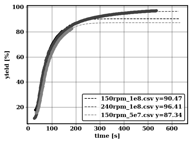
Perform early prediction
python applications/early_prediction.py -df bird/postprocess/data_early
Generates
Compute kLa with uncertainty estimates
Based on the time-history of the concentration of a species, one can calculate kLa by fitting the function
where \(C^*\) is the equilibrium concentration (to be fitted), \(C_0\) is the initial concentration, \(t\) is time, \(t_0\) is the initial time after which concentration is recorded
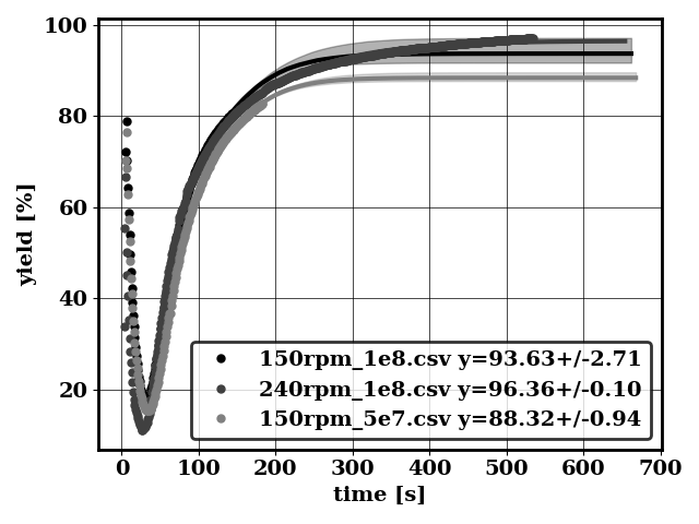
Accurate estimates can be obtained if sufficient data is acquired. Otherwise, it may be useful to derive uncertainty estimates about \(C^*\) and \(kLa\) (the parameters fitted)
This can be achieved with a Bayesian calibration procedure. The calibration is conducted by removing transient data, and by doing a data bootstrapping. The number of data to remove in the transient phase is automatically determined by examining how accurate is the fit.
python applications/compute_kla_uq.py -i bird/postprocess/data_kla/volume_avg.dat -ti 0 -ci 1 -mc 10
Generates
Chopping index = 0
Chopping index = 1
Chopping index = 2
Chopping index = 3
Chopping index = 4
Doing data bootstrapping
      scenario 0
      scenario 1
      scenario 2
      scenario 3
For bird/postprocess/data_kla/volume_avg.dat with time index: 0, concentration index: 1
     kla = 324 +/- 2.446 [h-1]
     cstar = 0.3107 +/- 0.0006522 [mol/m3]
Without data bootstrap
     kla = 324.5 +/- 2.075 [h-1]
     cstar = 0.3105 +/- 0.0005444 [mol/m3]
Compute mean statistics with uncertainty
Averaging a discretized time-series signal is used in many contexts to characterize bio reactors (to compute averaged holdup or species concentrations). Averaging is subject to statistical error and we provide tools to manage it.
The run the illustrative example we consider here:
python applications/compute_time_series_mean.py
There, we consider a time series acquired over the interval \([0, 2]\) where the signal is \(cos (2 \pi t)\) shown below
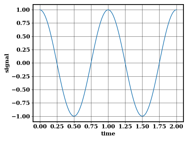
We can sample the signal with 100 points through the interval \([0, 2]\), and we obtain the following output
2025-09-02 12:36:15,016 [DEBUG] bird: Making the time series equally spaced over time
2025-09-02 12:36:15,016 [DEBUG] bird: Time series already equally spaced
2025-09-02 12:36:15,016 [DEBUG] bird: T0 = 1.270553916086648
2025-09-02 12:36:15,016 [INFO] bird: Mean = 0.01 +/- 0.081
The T0 value suggests that every \(1.27\) points is considered independent. The uncertainty about the mean is estimated via the central limit theorem, where the number of datapoints is downsampled to make the sample independents
We can also oversample the signal with 100 times more points. No more information has been provided about the signal, but without identifying the number of steps over which samples can be considered independent, the uncertainty (\(0.081\)) would be artificially reduced to \(0.0081\).
Here we obtain
2025-09-02 12:36:15,016 [DEBUG] bird: Making the time series equally spaced over time
2025-09-02 12:36:15,016 [DEBUG] bird: Time series already equally spaced
2025-09-02 12:36:15,030 [DEBUG] bird: T0 = 126.6515206796017
2025-09-02 12:36:15,030 [INFO] bird: Mean = 0.0001 +/- 0.08
The mean calculation function identifies that every 127 points is independent, and the uncertainty about the mean is not artificially reduced.