Parameter calibration for bubble size distribution (BSD)
This tutorial demonstrates how to calibrate bubble dynamics models by scaling the breakup and coalescence rates to match an observed BSD.
Running the tutorial
We assume that bird is installed within an environment called bird (see either the Installation section for developers or the Installation section for users)
You will need to install additional dependencies
conda activate bird
BIRD_DIR = `python -c "import bird; print(bird.BIRD_DIR)"`
cd ${BIRD_DIR}/../
pip install .[calibration]
The calibration tutorial is located at ${BIRD_DIR}/../tutorial_cases/calibration/bsd
Simple modeling of bubble size distribution (BSD) dynamics
In this example, the dynamics of the BSD are modeled for a frozen flow field, i.e. where the changes in BSD do not affect the fluid flow variables. Each bubble is modeled with a particle which can either be merged with another particle (coalescence) or be broken into multiple particles (breakup).
At every timestep, a number of breakup and coalescence events are determined by the breakup and coalescence rates.
In this example, breakup and coalescence rates are assumed independent of the bubble diameters. While simple, this implementation can result in a breakup or coalescence runaway in the case where breakup and coalescence rates are not balancing each other. In the case of breakup runaway, the number of particles grows monotonically, and in the base of coalescence runaway, the number of particles decreases monotonically.
For these runaway cases, the simulations are considered failing (see specific definition of failing in simulation.py.
At every event, we consider N-ary breakup and coalescence. If N=2, then the system models a binary breakup and binary coalescence: at every coalescence event, only two bubbles coalesce; at every breakup event, only two daughter bubbles are created starting from one initial bubble.
Calibration Objective
For all the cases, the simulation initially contains 2000 bubbles all with diameter 1mm.
Two target BSDs are considered:
A BSD obtained with a ternary breakup and coalescence with breakup and coalescence rate 0.5 Hz.
A BSD obtained with a binary breakup and coalescence with breakup rate 1.6 Hz and coalescence rate 2.0 Hz
Generate the target data by running
cd make_dataset
bash gen_target.sh
cd ..
This creates a folder data/ with the file target_n_3_br_0.5_cr_0.5.npz and target_n_2_br_1.6_cr_2.0.npz
The numerical model is always a binary breakup and coalescence model with adjustable breakup and coalescence rate. To avoid breakup or coalescence runaway, we ensure that breakup rate is close to the coalescence rate. Specifically, the coalescence rate Cr varies in the interval [0.02, 2]. A breakup rate factor Bf varies in the interval [0.8, 1.1] and the breakup rate Br = Bf Cr. This ensures that the breakup rate and coalescence rate are close to one another, thereby avoiding breakup and coalescence runaway.
Each simulation (target and from the numerical model) uses a timeste dt = 0.01s and the simulations are run for 150s to reach statistical stationarity and allow for sufficient averaging of the BSD. Since each forward simulation is expensive (~30s on a M1 Mac), a surrogate needs to be constructed.
Building the surrogate
The class Param_NN available in BiRD allows to create a parametric surrogate. Here, the input of the surrogate are the parameters beff_fact (corresponding to Bf as defined above) and ceff (corresponding to Cr as defined above), and the variable x that parameterize the PDF (the bubble diameter).
Generate dataset
cd make_dataset
bash gen_dataset.sh
cd ..
This generates a file data/dataset.npz that contains the BSD of 400 simulations. This step may take time (~3h on a M1 Mac). We provide a dataset.npz that contains precomputed BSD.
Before moving further, we can plot the data to understand how close it is to the target data and whether it is subject to coalescence and breakup runaway.
cd data
python check_real.py -ter
cd ..
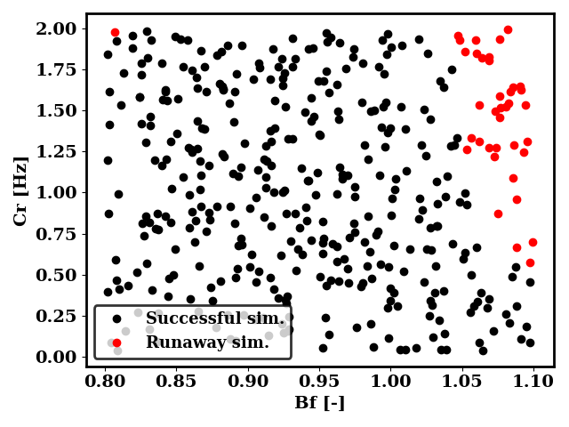
The plot below shows the values of Bf and Cr simulated and whether they lead to runaway. Most of the simulations are successful, but very small and very large values of Bf lead to runaway. Those runs are labelled with a dummy PDF in order to instruct the surrogate model to avoid those regions
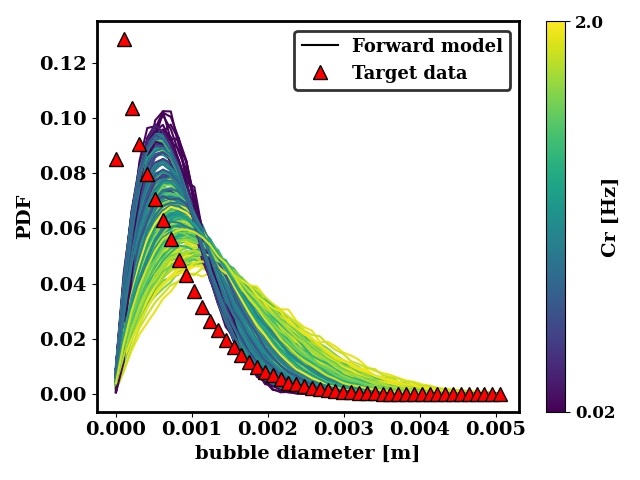
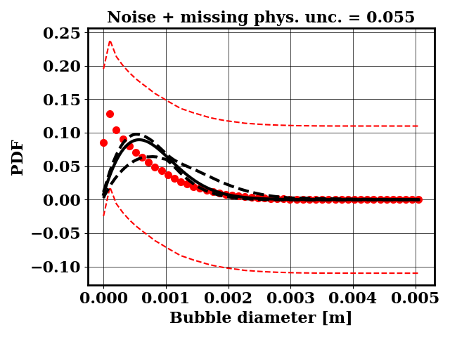
We can also look at how close the generated data is to the target data. For the ternary breakup and coalescence, there is clearly a discrepancy that is not resolvable by adjusting the coalescence and breakup rates.
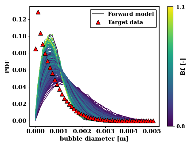
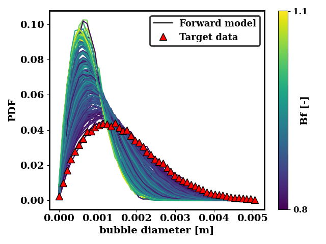
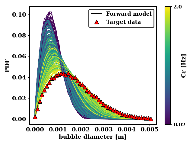
In the case of the binary breakup and coalescence target data, a low value of Bf and a high value of Cr should lead to a good agreement between the forward model and the target data.
Train a neural net surrogate
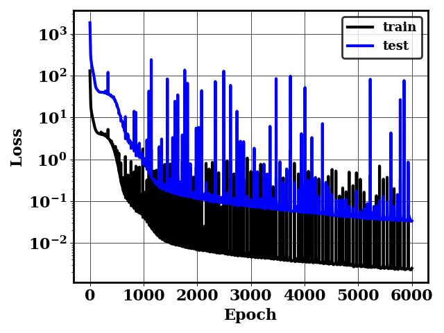
bash train_surrogate.sh
This will generate a plot of the train and test loss history loss.png. This will also generate Modeltmp which contains the weights of the trained model and Logtmp which contains the loss history (shown below).
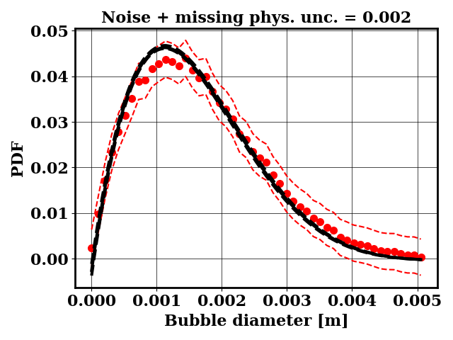
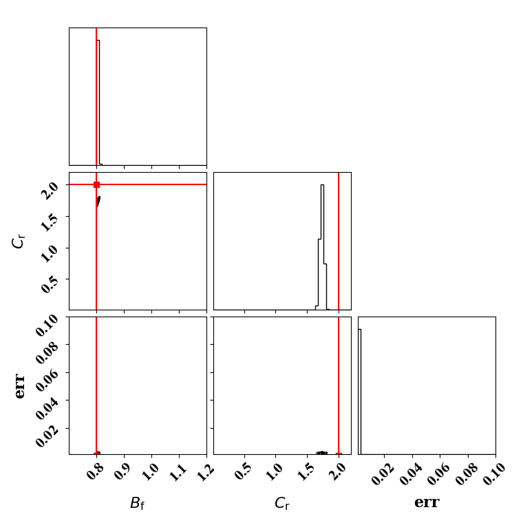
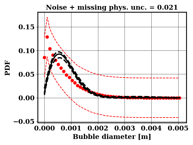
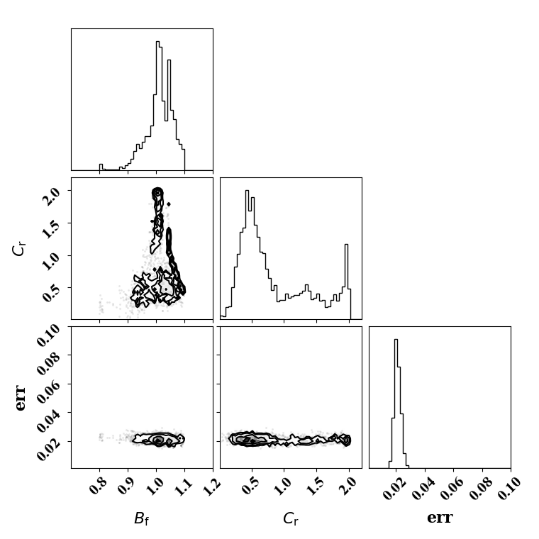
Calibration with optimized likelihood uncertainty
For the calibration, the objective PDF is noisy and subject to statistical uncertainty. We calibrate a likelihood uncertainty that contains both the noise and the missing physics estimates.
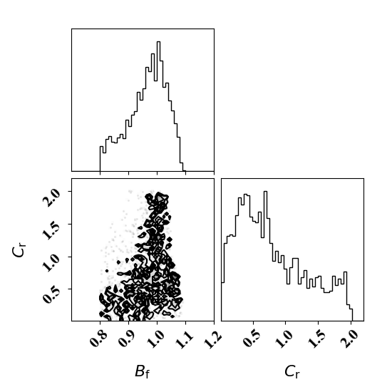
Calibrate against the target data obtained with ternary breakup and coalescence
python tut_calibration.py -ter
Calibrate against the target data obtained with binary breakup and coalescence
python tut_calibration.py
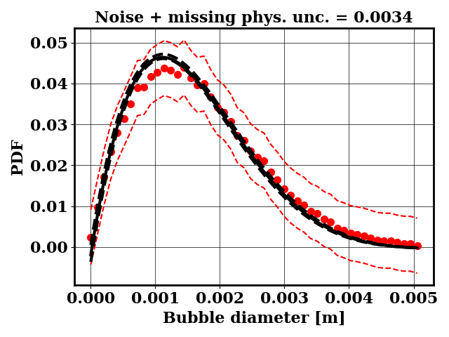
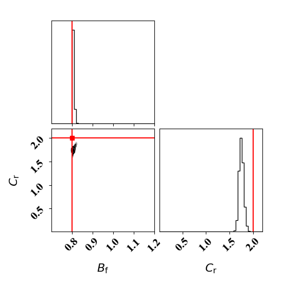
Clearly, the amount of missing physics vary depending on the observations and is significantly lower when calibrating against binary breakup and coalescence data.
Calibration with calibrated likelihood uncertainty
The same suite of tests can be done by calibrating the likelihood uncertainty in lieu of optimizing it. This has the advantage of rapid calibration since only one calibration is needed.
Calibrate against the target data obtained with ternary breakup and coalescence
python tut_calibration.py -ter -cal_err
Calibrate against the target data obtained with binary breakup and coalescence
python tut_calibration.py -cal_err