LETID - Accelerated Tests#
Several standardized accelerated tests have been developed for LETID. These include IEC TS 63342 for c-Si photovoltaic modules, and IEC TS 63202-4 for c-Si photovoltaic cells. Both procedures essentially prescribe exposure to constant light or current injection at constant elevated temperature for a prescribed duration of time. This notebook demonstrates how to use this library to model device behavior in such a procedure.
Requirements:
pandas,numpy,matplotlib
Objectives:
Define necessary solar cell device parameters
Define necessary degradation parameters: degraded lifetime and defect states
Create timeseries of temperature and current injection
Run through timeseries, calculating defect states
Calculate device degradation and plot
# if running on google colab, uncomment the next line and execute this cell to install the dependencies and prevent "ModuleNotFoundError" in later cells:
# !pip install pvdeg==0.3.3
from pvdeg import letid, collection, utilities, DATA_DIR

import os
import pandas as pd
import numpy as np
import matplotlib.pyplot as plt
import pvdeg
import datetime as dt
# This information helps with debugging and getting support :)
import sys
import platform

print("Working on a ", platform.system(), platform.release())
print("Python version ", sys.version)
print("Pandas version ", pd.__version__)
print("pvdeg version ", pvdeg.__version__)
Working on a  Linux 6.11.0-1018-azure
Python version  3.11.13 (main, Jun  4 2025, 04:12:12) [GCC 13.3.0]
Pandas version  2.3.3
pvdeg version  0.1.dev1+g51172fdc5
Device parameters#
To define a device, we need to define several important quantities about the device: wafer thickness (in \(\mu m\)), rear surface recombination velocity (in cm/s), and cell area (in cm2). The values defined below are representative of a typical PERC solar cell.
wafer_thickness = 180  # um
s_rear = 46  # cm/s
cell_area = 243  # cm^2
Other device parameters#
Other required device parameters: base diffusivity (in \(cm^2/s\)), and optical generation profile, which allow us to estimate current collection in the device.
generation_df = pd.read_excel(
    os.path.join(DATA_DIR, "PVL_GenProfile.xlsx"), header=0
)  # this is an optical generation profile generated by PVLighthouse's OPAL2 default model for 1-sun, normal incident AM1.5 sunlight on a 180-um thick SiNx-coated, pyramid-textured wafer.
generation = generation_df["Generation (cm-3s-1)"]
depth = generation_df["Depth (um)"]

d_base = 27  # cm^2/s electron diffusivity. See https://www2.pvlighthouse.com.au/calculators/mobility%20calculator/mobility%20calculator.aspx for details
Degradation parameters#
To model the device’s degradation, we need to define several more important quantities about the degradation the device will experience. These include undegraded and degraded lifetime (in \(\mu s\)).
tau_0 = 115  # us, carrier lifetime in non-degraded states, e.g. LETID/LID states A or C
tau_deg = 55  # us, carrier lifetime in fully-degraded state, e.g. LETID/LID state B
Let’s see how much maximum power degradation these parameters will result in:
loss, pmp_0, pmp_deg = letid.calc_pmp_loss_from_tau_loss(
    tau_0, tau_deg, cell_area, wafer_thickness, s_rear
)  # returns % power loss, pmp_0, pmp_deg
print(loss)
0.03495240755084558
Check to see the device’s current collection
jsc_0 = collection.calculate_jsc_from_tau_cp(
    tau_0, wafer_thickness, d_base, s_rear, generation, depth
)  # returns short-circuit current (Jsc) in mA/cm^2 given required cell parameters
print(jsc_0)
41.59099692285122
Remaining degradation parameters:
The rest of the quantities to define are: the initial percentage of defects in each state (A, B, and C), and the dictionary of mechanism parameters.
In this example, we’ll assume the device starts in the fully-undegraded state (100% state A), and we’ll use the parameters for LETID degradation from Repins.
# starting defect state percentages
nA_0 = 100
nB_0 = 0
nC_0 = 0
# Here's a list of the possible sets of kinetic parameters from kinetic_parameters.json:
utilities.get_kinetics()
('Choose a set of kinetic parameters:',
 ['repins',
  'repins_best_case',
  'kwapil',
  'bredemeier',
  'wyller_wafer',
  'wyller_cell',
  'graf',
  'dark letid',
  'bo-lid',
  'Lit BO-LID + fit to Qcells destab'])
mechanism_params = utilities.get_kinetics("repins")
print(mechanism_params)
{'mechanism': 'LETID', 'v_ab': 46700000.0, 'v_ba': 4.7e-25, 'v_bc': 19900000.0, 'v_cb': 0.0, 'ea_ab': 0.827, 'ea_ba': -1.15, 'ea_bc': 0.871, 'ea_cb': 0.0, 'suns_ab': 1.0, 'suns_bc': 1.0, 'temperature_ab': 410, 'temperature_bc': 410, 'tau_ab': 75, 'tau_bc': 75, 'x_ab': 1, 'x_ba': 1.7, 'x_bc': 1.2, 'structure_ab': 'cell', 'structure_bc': 'cell', 'thickness_ab': 200, 'thickness_bc': 200, 'srv_ab': 90, 'srv_bc': 90, 'doi': 'doi:10.1557/s43577-022-00438-8', 'comments': ''}
Set up timeseries#
In this example, we are going to model test with constant temperature and current injection. IEC TS 63342 prescribes two to three weeks of injection equivalent to \(2\times(I_{sc}-I_{mp})\), at \(75\degree C\). For most typical c-Si modules, \(2\times(I_{sc}-I_{mp})\) is roughly equal to \(0.1\times I_{sc}\). So we will set injection equal to 0.1 “suns” of injection.
We will create a pandas datetime series and calculate the changes in defect states for each timestep.
temperature = 75  # degrees celsius
suns = 0.1  # "suns" of injection, e.g 1-sun illumination at open circuit would be 1; dark current injection is given as a fraction of Isc, e.g., injecting Isc would be 1. For this example we assume injection is 0.1*Isc.

duration = "3W"
freq = "min"
start = "2022-01-01"

# default is 3 weeks of 1-minute interval timesteps. In general, we should select small timesteps unless we are sure defect reactions are proceeding very slowly
timesteps = pd.date_range(
    start, end=pd.to_datetime(start) + pd.to_timedelta(duration), freq=freq
)
timesteps = pd.DataFrame(timesteps, columns=["Datetime"])


temps = np.full(len(timesteps), temperature)
injection = np.full(len(timesteps), suns)

timesteps["Temperature"] = temps
timesteps["Injection"] = injection

timesteps[["NA", "NB", "NC", "tau"]] = (
    np.nan
)  # create columns for defect state percentages and lifetime, fill with NaNs for now, to fill iteratively below

timesteps.loc[0, ["NA", "NB", "NC"]] = (
    nA_0,
    nB_0,
    nC_0,
)  # assign first timestep defect state percentages
timesteps.loc[0, "tau"] = letid.tau_now(
    tau_0, tau_deg, nB_0
)  # calculate tau for the first timestep
timesteps
| Datetime | Temperature | Injection | NA | NB | NC | tau | |
|---|---|---|---|---|---|---|---|
| 0 | 2022-01-01 00:00:00 | 75 | 0.1 | 100.0 | 0.0 | 0.0 | 115.0 |
| 1 | 2022-01-01 00:01:00 | 75 | 0.1 | NaN | NaN | NaN | NaN |
| 2 | 2022-01-01 00:02:00 | 75 | 0.1 | NaN | NaN | NaN | NaN |
| 3 | 2022-01-01 00:03:00 | 75 | 0.1 | NaN | NaN | NaN | NaN |
| 4 | 2022-01-01 00:04:00 | 75 | 0.1 | NaN | NaN | NaN | NaN |
| ... | ... | ... | ... | ... | ... | ... | ... |
| 30236 | 2022-01-21 23:56:00 | 75 | 0.1 | NaN | NaN | NaN | NaN |
| 30237 | 2022-01-21 23:57:00 | 75 | 0.1 | NaN | NaN | NaN | NaN |
| 30238 | 2022-01-21 23:58:00 | 75 | 0.1 | NaN | NaN | NaN | NaN |
| 30239 | 2022-01-21 23:59:00 | 75 | 0.1 | NaN | NaN | NaN | NaN |
| 30240 | 2022-01-22 00:00:00 | 75 | 0.1 | NaN | NaN | NaN | NaN |
30241 rows × 7 columns
Run through timesteps#
Since each timestep depends on the preceding timestep, we need to calculate in a loop. This will take a few minutes depending on the length of the timeseries.
for index, timestep in timesteps.iterrows():
    # first row tau has already been assigned
    if index == 0:
        pass

    # loop through rows, new tau calculated based on previous NB. Reaction proceeds based on new tau.
    else:
        n_A = timesteps.at[index - 1, "NA"]
        n_B = timesteps.at[index - 1, "NB"]
        n_C = timesteps.at[index - 1, "NC"]

        tau = letid.tau_now(tau_0, tau_deg, n_B)
        jsc = collection.calculate_jsc_from_tau_cp(
            tau, wafer_thickness, d_base, s_rear, generation, depth
        )

        temperature = timesteps.at[index, "Temperature"]
        injection = timesteps.at[index, "Injection"]

        # calculate defect reaction kinetics: reaction constant and carrier concentration factor.
        k_AB = letid.k_ij(
            mechanism_params["v_ab"], mechanism_params["ea_ab"], temperature
        )
        k_BA = letid.k_ij(
            mechanism_params["v_ba"], mechanism_params["ea_ba"], temperature
        )
        k_BC = letid.k_ij(
            mechanism_params["v_bc"], mechanism_params["ea_bc"], temperature
        )
        k_CB = letid.k_ij(
            mechanism_params["v_cb"], mechanism_params["ea_cb"], temperature
        )

        x_ab = letid.carrier_factor(
            tau,
            "ab",
            temperature,
            injection,
            jsc,
            wafer_thickness,
            s_rear,
            mechanism_params,
        )
        x_ba = letid.carrier_factor(
            tau,
            "ba",
            temperature,
            injection,
            jsc,
            wafer_thickness,
            s_rear,
            mechanism_params,
        )
        x_bc = letid.carrier_factor(
            tau,
            "bc",
            temperature,
            injection,
            jsc,
            wafer_thickness,
            s_rear,
            mechanism_params,
        )

        # calculate the instantaneous change in NA, NB, and NC
        dN_Adt = (k_BA * n_B * x_ba) - (k_AB * n_A * x_ab)
        dN_Bdt = (
            (k_AB * n_A * x_ab) + (k_CB * n_C) - ((k_BA * x_ba + k_BC * x_bc) * n_B)
        )
        dN_Cdt = (k_BC * n_B * x_bc) - (k_CB * n_C)

        t_step = (
            timesteps.at[index, "Datetime"] - timesteps.at[index - 1, "Datetime"]
        ).total_seconds()

        # assign new defect state percentages
        timesteps.at[index, "NA"] = n_A + dN_Adt * t_step
        timesteps.at[index, "NB"] = n_B + dN_Bdt * t_step
        timesteps.at[index, "NC"] = n_C + dN_Cdt * t_step
---------------------------------------------------------------------------
KeyboardInterrupt                         Traceback (most recent call last)
/tmp/ipykernel_2468/1706429461.py in ?()
      9         n_B = timesteps.at[index - 1, "NB"]
     10         n_C = timesteps.at[index - 1, "NC"]
     11
     12         tau = letid.tau_now(tau_0, tau_deg, n_B)
---> 13         jsc = collection.calculate_jsc_from_tau_cp(
     14             tau, wafer_thickness, d_base, s_rear, generation, depth
     15         )
     16

/opt/hostedtoolcache/Python/3.11.13/x64/lib/python3.11/site-packages/pvdeg/collection.py in ?(tau, wafer_thickness, d_base, s_rear, generation, depth, w_emitter, l_emitter, d_emitter, s_emitter, xp)
    183     cp_depletion = np.ones(len(depletion_depth))
    184
    185     cp_base = collection_probability(base_depth, w_base, s_base, l_base, d_base)
    186
--> 187     depth_array = np.concatenate(
    188         np.array([emitter_depth, depletion_depth, base_depth], dtype=object), axis=0
    189     )
    190     collection_array = np.concatenate(

/opt/hostedtoolcache/Python/3.11.13/x64/lib/python3.11/site-packages/pandas/core/generic.py in ?(self, name)
-> 6306     @final
   6307     def __getattr__(self, name: str):
   6308         """
   6309         After regular attribute access, try looking up the name

KeyboardInterrupt:
Finish calculating degraded device parameters.#
Now that we have calculated defect states, we can calculate all the quantities that depend on defect states.
timesteps["tau"] = letid.tau_now(tau_0, tau_deg, timesteps["NB"])

# calculate device Jsc for every timestep. Unfortunately this requires an integration so I think we have to run through a loop. Device Jsc allows calculation of device Voc.
for index, timestep in timesteps.iterrows():
    jsc_now = collection.calculate_jsc_from_tau_cp(
        timesteps.at[index, "tau"], wafer_thickness, d_base, s_rear, generation, depth
    )
    timesteps.at[index, "Jsc"] = jsc_now
    timesteps.at[index, "Voc"] = letid.calc_voc_from_tau(
        timesteps.at[index, "tau"], wafer_thickness, s_rear, jsc_now, temperature=25
    )
# this function quickly calculates the rest of the device parameters: Isc, FF, max power, and normalized max power
timesteps = letid.calc_device_params(timesteps, cell_area=243)
timesteps["time (days)"] = (
    timesteps["Datetime"] - timesteps.iloc[0]["Datetime"]
).dt.total_seconds() / 86400  # create a column for days elapsed

timesteps
| Datetime | Temperature | Injection | NA | NB | NC | tau | Jsc | Voc | Isc | FF | Pmp | Pmp_norm | time (days) | |
|---|---|---|---|---|---|---|---|---|---|---|---|---|---|---|
| 0 | 2022-01-01 00:00:00 | 75 | 0.1 | 100.000000 | 0.000000 | 0.000000 | 115.000000 | 41.590997 | 0.666327 | 10.106612 | 0.840987 | 5.663467 | 1.000000 | 0.000000 |
| 1 | 2022-01-01 00:01:00 | 75 | 0.1 | 99.945424 | 0.054576 | 0.000000 | 114.931573 | 41.590784 | 0.666316 | 10.106561 | 0.840985 | 5.663325 | 0.999975 | 0.000694 |
| 2 | 2022-01-01 00:02:00 | 75 | 0.1 | 99.890904 | 0.109094 | 0.000002 | 114.863300 | 41.590572 | 0.666304 | 10.106509 | 0.840983 | 5.663184 | 0.999950 | 0.001389 |
| 3 | 2022-01-01 00:03:00 | 75 | 0.1 | 99.836439 | 0.163555 | 0.000006 | 114.795178 | 41.590359 | 0.666292 | 10.106457 | 0.840981 | 5.663043 | 0.999925 | 0.002083 |
| 4 | 2022-01-01 00:04:00 | 75 | 0.1 | 99.782028 | 0.217959 | 0.000012 | 114.727209 | 41.590147 | 0.666281 | 10.106406 | 0.840979 | 5.662902 | 0.999900 | 0.002778 |
| ... | ... | ... | ... | ... | ... | ... | ... | ... | ... | ... | ... | ... | ... | ... |
| 30236 | 2022-01-21 23:56:00 | 75 | 0.1 | 0.006066 | 54.974093 | 45.019841 | 71.887698 | 41.381392 | 0.656754 | 10.055678 | 0.839286 | 5.542735 | 0.978682 | 20.997222 |
| 30237 | 2022-01-21 23:57:00 | 75 | 0.1 | 0.006065 | 54.972773 | 45.021162 | 71.888345 | 41.381397 | 0.656754 | 10.055679 | 0.839286 | 5.542738 | 0.978683 | 20.997917 |
| 30238 | 2022-01-21 23:58:00 | 75 | 0.1 | 0.006064 | 54.971454 | 45.022482 | 71.888992 | 41.381402 | 0.656754 | 10.055681 | 0.839286 | 5.542740 | 0.978683 | 20.998611 |
| 30239 | 2022-01-21 23:59:00 | 75 | 0.1 | 0.006063 | 54.970135 | 45.023802 | 71.889638 | 41.381407 | 0.656755 | 10.055682 | 0.839286 | 5.542743 | 0.978684 | 20.999306 |
| 30240 | 2022-01-22 00:00:00 | 75 | 0.1 | 0.006061 | 54.968816 | 45.025123 | 71.890285 | 41.381411 | 0.656755 | 10.055683 | 0.839286 | 5.542745 | 0.978684 | 21.000000 |
30241 rows × 14 columns
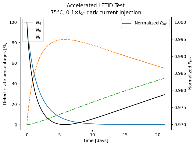
Plot the results#
from cycler import cycler

plt.style.use("default")

fig, ax = plt.subplots()

ax.set_prop_cycle(
    cycler("color", ["tab:blue", "tab:orange", "tab:green"])
    + cycler("linestyle", ["-", "--", "-."])
)

ax.plot(timesteps["time (days)"], timesteps[["NA", "NB", "NC"]].values)

ax.legend(labels=["$N_A$", "$N_B$", "$N_C$", "80 % regeneration"], loc="upper left")
ax.set_ylabel("Defect state percentages [%]")
ax.set_xlabel("Time [days]")

ax2 = ax.twinx()
ax2.plot(
    timesteps["time (days)"],
    timesteps["Pmp_norm"],
    c="black",
    label="Normalized $P_{MP}$",
)
ax2.legend(loc="upper right")
ax2.set_ylabel("Normalized $P_{MP}$")

# ax.axvline(pvdeg.Degradation.calc_regeneration_time(timesteps).total_seconds()/(60*60*24), linestyle = ':' , c = 'grey')
# ax.annotate('80% regeneration', (pvdeg.Degradation.calc_regeneration_time(timesteps).total_seconds()/(60*60*24), 80),
#            xytext=(0.5, 0.8), textcoords='axes fraction',
#            arrowprops=dict(facecolor='black', shrink=0.1),
#            horizontalalignment='right', verticalalignment='top')

ax.set_title(
    "Accelerated LETID Test\n"
    rf"{temperature}$\degree$C, {suns}$\times I_{{SC}}$ dark current injection"
)

plt.show()
The function calc_letid_lab wraps all of the steps above into a single function:
FIXED_START_DATE = dt.datetime(2025, 9, 9, 0, 0)
result = letid.calc_letid_lab(
    tau_0, tau_deg, wafer_thickness, s_rear, nA_0, nB_0, nC_0, 0.1, 75, "repins",
    start=FIXED_START_DATE
)
result["Datetime"] = result["Datetime"].dt.round("s")
print(result)
                 Datetime  Temperature  Injection          NA         NB  \
0     2025-09-09 00:00:00           75        0.1  100.000000   0.000000
1     2025-09-09 00:01:00           75        0.1   99.945424   0.054576
2     2025-09-09 00:02:00           75        0.1   99.890904   0.109094
3     2025-09-09 00:03:00           75        0.1   99.836439   0.163555
4     2025-09-09 00:04:00           75        0.1   99.782028   0.217959
...                   ...          ...        ...         ...        ...
30236 2025-09-29 23:56:00           75        0.1    0.006066  54.974093
30237 2025-09-29 23:57:00           75        0.1    0.006065  54.972773
30238 2025-09-29 23:58:00           75        0.1    0.006064  54.971454
30239 2025-09-29 23:59:00           75        0.1    0.006063  54.970135
30240 2025-09-30 00:00:00           75        0.1    0.006061  54.968816

              NC         tau        Jsc       Voc       Isc        FF  \
0       0.000000  115.000000  41.590997  0.666327  9.940248  0.840987
1       0.000000  114.931573  41.590997  0.666327  9.940248  0.840987
2       0.000002  114.863300  41.590784  0.666316  9.940197  0.840985
3       0.000006  114.795178  41.590572  0.666304  9.940147  0.840983
4       0.000012  114.727209  41.590359  0.666292  9.940096  0.840981
...          ...         ...        ...       ...       ...       ...
30236  45.019841   71.887698  41.381387  0.656754  9.890151  0.839286
30237  45.021162   71.888345  41.381392  0.656754  9.890153  0.839286
30238  45.022482   71.888992  41.381397  0.656754  9.890154  0.839286
30239  45.023802   71.889638  41.381402  0.656754  9.890155  0.839286
30240  45.025123   71.890285  41.381407  0.656755  9.890156  0.839286

            Pmp  Pmp_norm
0      5.570241  1.000000
1      5.570241  1.000000
2      5.570102  0.999975
3      5.569963  0.999950
4      5.569824  0.999925
...         ...       ...
30236  5.451494  0.978682
30237  5.451497  0.978682
30238  5.451499  0.978683
30239  5.451502  0.978683
30240  5.451504  0.978684

[30241 rows x 13 columns]