Temperature Models Example

This example demonstrates how to use models with temperature as a feature in the Routee Powertrain library.

import nrel.routee.powertrain as pt
import pandas as pd
import matplotlib.pyplot as plt

2025-10-24 16:16:13,049 [INFO] - Failed to extract font properties from /usr/share/fonts/truetype/noto/NotoColorEmoji.ttf: Can not load face (unknown file format; error code 0x2)

2025-10-24 16:16:13,394 [INFO] - generated new fontManager

To demonstrate the use of temperature models, we will load a standard Tesla Model 3 RWD model (without temperature as a feature) and two temperature models (steady-state and transient) for the same vehicle. We will then predict energy consumption over a sample route at different ambient temperatures (72°F and 32°F) and compare the results.

It's important to understand the distinction between steady-state and transient temperature models:

• Steady-State Temperature Models: These models assume that the vehicle's thermal conditions have stabilized to a constant state. They are typically used for longer trips where the vehicle has had sufficient time for the control systems to have stabilized the thermal environment. In this example, we will use the steady-state model for the portion of the trip after the first 5 minutes at 32°F.

• Transient Temperature Models: These models account for the period when the vehicle is still adjusting to the ambient temperature. For example, when a vehicle starts a trip in cold weather and has been sitting outside, it takes some time for the battery and cabin to warm up.

tesla = pt.load_model("2022_Tesla_Model_3_RWD")
tesla_with_temp_steady = pt.load_model("2022_Tesla_Model_3_RWD_0F_110F_steady")
tesla_with_temp_transient = pt.load_model("2022_Tesla_Model_3_RWD_0F_110F_transient")

Load a sample route and prepare it for prediction.

sample_route = pt.load_sample_route()
sample_route["time_minutes"] = (
    sample_route["distance"] / sample_route["speed_mph"]
) * 60
sample_route["cummulative_time_minutes"] = sample_route["time_minutes"].cumsum()
sample_route["cummulative_distance"] = sample_route["distance"].cumsum()

Set the ambient temperature for the route.

sample_route_72F = sample_route.copy()
sample_route_72F["ambient_temp_f"] = 72

sample_route_32F = sample_route.copy()
sample_route_32F["ambient_temp_f"] = 32

For the 32°F route, we will use the transient model for the first 5 minutes and the steady-state model for the remainder of the trip.

sample_route_32F_transient = sample_route_32F[
    sample_route_32F["cummulative_time_minutes"] <= 5
]
sample_route_32F_steady = sample_route_32F[
    sample_route_32F["cummulative_time_minutes"] > 5
]

Predict energy consumption using the different models and ambient temperatures.

energy = tesla.predict(sample_route, feature_columns=["speed_mph", "grade_percent"])
energy_with_temp_72F = tesla_with_temp_steady.predict(
    sample_route_72F, feature_columns=["speed_mph", "grade_percent", "ambient_temp_f"]
)
energy_with_temp_32F_transient = tesla_with_temp_transient.predict(
    sample_route_32F_transient,
    feature_columns=["speed_mph", "grade_percent", "ambient_temp_f"],
)
energy_with_temp_32F_steady = tesla_with_temp_steady.predict(
    sample_route_32F_steady,
    feature_columns=["speed_mph", "grade_percent", "ambient_temp_f"],
)
energy_with_temp_32F = pd.concat(
    [energy_with_temp_32F_transient, energy_with_temp_32F_steady]
)

Now, we can compare the energy consumption results.

energy["cummulative_energy_kwh"] = energy["kwh"].cumsum()
energy_with_temp_72F["cummulative_energy_kwh"] = energy_with_temp_72F["kwh"].cumsum()
energy_with_temp_32F["cummulative_energy_kwh"] = energy_with_temp_32F["kwh"].cumsum()
plt.plot(
    sample_route["cummulative_distance"],
    energy["cummulative_energy_kwh"],
    label="Tesla without Temperature",
)
plt.plot(
    sample_route["cummulative_distance"],
    energy_with_temp_72F["cummulative_energy_kwh"],
    label="Tesla with Temperature 72F",
)
plt.plot(
    sample_route["cummulative_distance"],
    energy_with_temp_32F["cummulative_energy_kwh"],
    label="Tesla with Temperature 32F",
)
plt.xlabel("Cumulative Distance (miles)")
plt.ylabel("Cumulative Energy (kWh)")
plt.legend()

<matplotlib.legend.Legend at 0x7f3658940b50>

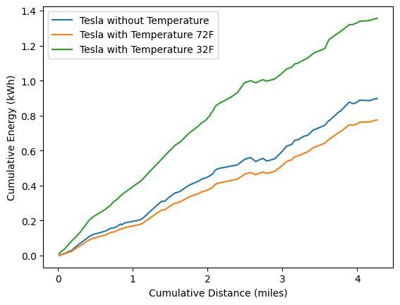
Notice how the energy consumption for the 32°F route is higher than the other two scenarios, reflecting the increased energy demand in colder temperatures.

Something else to note is that the model that doesn't consider temperature explicitly includes a "real world correction factor" to account for things like temperature on average. This explains why the energy consumption for the 72°F route is slightly lower than the other two scenarios since the model without temperature adjustment is effectively averaging out the impact of temperature. The 72°F condition would be considered the "ideal" case since the vehicle does not have to expand any extra effort to maintain the cabin temperature.

Multi-Vehicle Comparison

Now let's compare the Tesla Model 3 with other electric vehicles to see how different EVs perform under various temperature conditions. We'll load the Nissan Leaf and Chevrolet Bolt models and compare their energy consumption across different temperatures.

# Load Nissan Leaf models
nissan_leaf_steady = pt.load_model("2016_Nissan_Leaf_30_kWh_0F_110F_steady")
nissan_leaf_transient = pt.load_model("2016_Nissan_Leaf_30_kWh_0F_110F_transient")

# Load Chevrolet Bolt models
chevy_bolt_steady = pt.load_model("2020_Chevrolet_Bolt_EV_0F_110F_steady")
chevy_bolt_transient = pt.load_model("2020_Chevrolet_Bolt_EV_0F_110F_transient")

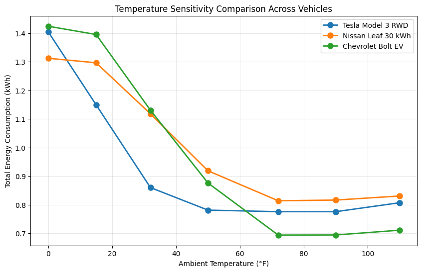
Temperature Sensitivity Comparison

Let's compare how each vehicle's energy consumption changes across a range of temperatures (0°F, 15°F, 32°F, 50°F, 72°F, 90°F, 110°F). We'll use steady-state models for this comparison.

# Predict energy for all vehicles at different temperatures
temperatures = [0, 15, 32, 50, 72, 90, 110]
vehicles_data = {
    "Tesla Model 3 RWD": tesla_with_temp_steady,
    "Nissan Leaf 30 kWh": nissan_leaf_steady,
    "Chevrolet Bolt EV": chevy_bolt_steady,
}

total_energy_by_temp = {vehicle: [] for vehicle in vehicles_data.keys()}

for temp in temperatures:
    route_temp = sample_route.copy()
    route_temp["ambient_temp_f"] = temp

    for vehicle_name, model in vehicles_data.items():
        energy_pred = model.predict(
            route_temp, feature_columns=["speed_mph", "grade_percent", "ambient_temp_f"]
        )
        total_energy_by_temp[vehicle_name].append(energy_pred["kwh"].sum())

# Create temperature sensitivity comparison plot
plt.figure(figsize=(10, 6))
for vehicle_name, energies in total_energy_by_temp.items():
    plt.plot(
        temperatures,
        energies,
        marker="o",
        linewidth=2,
        markersize=8,
        label=vehicle_name,
    )

plt.xlabel("Ambient Temperature (°F)")
plt.ylabel("Total Energy Consumption (kWh)")
plt.title("Temperature Sensitivity Comparison Across Vehicles")
plt.legend()
plt.grid(True, alpha=0.3)