TF-MELT Utilities Subpackage

This package contains utility functions for data processing, evaluation, visualization, and other common tasks in machine learning. The subpackage is organized into the following modules:

• Evaluation Module: Functions for evaluating model performance. Includes functions for making predictions for standard and ensemble models.

• Preprocessing Module: Functions for data preprocessing. Includes functions for normalizing data built on Scikit-learn normalizers.

• Statistics Module: Functions for computing statistics on data. Includes functions for computing metrics for uncertainty quantification.

• Visualization Module: Functions for visualizing data. Includes functions for plotting data, model predictions, and uncertainty metrics.

Evaluation Module

tfmelt.utils.evaluation.ensemble_predictions(model, x_data, y_normalizer: Any | None = None, unnormalize: bool | None = False, n_iter: int | None = 100, training: bool | None = False)

Make ensemble predictions using the provided model and optionally unscale the results. This is useful for models with probabilistic evaluation such as Bayesian Neural Networks or Artificial Neural Networks using Monte Carlo Dropout.

Parameters:

• model – The trained model to use for making predictions.

• x_data (array-like) – Data features to make predictions on.

• y_normalizer (optional) – The normalizer used for the target variable, to unscale the predictions. Defaults to None.

• unnormalize (bool) – Whether to unscale the predictions using the y_normalizer. Defaults to False.

• n_iter (int) – Number of iterations for ensemble predictions. Defaults to 100.

• training (bool) – Whether to use training mode for making predictions. Defaults to False.

Returns:

Mean and standard deviation of predictions (unnormalized if specified).

Return type:

tuple

tfmelt.utils.evaluation.extract_statistics_from_pdf(model, x_data, y_normalizer: Any | None = None, unnormalize: bool | None = False)

Extract statistics from the model’s PDF predictions and optionally unscale the results. This is useful for models that output a distribution as the prediction, such as a Bayesian Neural Network with aleatoric uncertainty enabled.

Parameters:

• model – The trained model to use for making predictions.

• x_data (array-like) – Data features to make predictions on.

• y_normalizer (optional) – The normalizer used for the target variable, to unscale the predictions. Defaults to None.

• unnormalize (bool) – Whether to unscale the predictions using the y_normalizer. Defaults to False.

Returns:

Mean and standard deviation of predictions (unnormalized if specified).

Return type:

tuple

tfmelt.utils.evaluation.make_predictions(model, x_data, y_normalizer: Any | None = None, unnormalize: bool | None = False, training: bool | None = False)

Make predictions using the provided model and optionally unscale the results.

Parameters:

• model – The trained model to use for making predictions.

• x_data (array-like) – Data features to make predictions on.

• y_normalizer (scaler, optional) – The normalizer used for the target variable, to unscale the predictions. Defaults to None.

• unnormalize (bool, optional) – Whether to unscale the predictions using the y_normalizer. Defaults to False.

• training (bool, optional) – Whether to use training mode for making predictions. Defaults to False.

Returns:

Predictions (unnormalized if specified).

Return type:

array-like

Preprocessing Module

class tfmelt.utils.preprocessing.IdentityScaler(**kwargs)

Bases: object

A scaler that performs no scaling, behaving like an identity function.

This class is useful for pipelines where a scaler is optional, but the pipeline expects a fit and transform method to be present like in Scikit-learn.

fit(X, y: Any | None = None)

Dummy fit method that does nothing.

Parameters:

• X (array-like) – Input data.

• y (array-like) – Ignored.

fit_transform(X, y: Any | None = None)

Dummy fit_transform method that returns the input data unchanged.

Parameters:

• X (array-like) – Input data.

• y (array-like) – Ignored.

inverse_transform(X)

Dummy inverse_transform method that returns the input data unchanged.

Parameters:

X (array-like) – Input data.

transform(X)

Dummy transform method that returns the input data unchanged.

Parameters:

X (array-like) – Input data.

tfmelt.utils.preprocessing.get_normalizers(norm_type: str | None = 'standard', n_normalizers: int | None = 1, **kwargs)

Get a list of normalizers based on the specified normalization type and number of normalizers.

Parameters:

• norm_type (str, optional) – Type of normalization (‘standard’, ‘minmax’,

• 'robust'

• 'power'

• 'standard'. ('quantile'). Defaults to)

• n_normalizers (int, optional) – Number of normalizers to create. Defaults to 1.

• **kwargs – Additional keyword arguments for the specific scaler.

Returns:

A list of normalizers.

Return type:

list

Statistics Module

tfmelt.utils.statistics.compute_crps(truth, mean, std)

Compute the continuous ranked probability score (CRPS) assuming a Gaussian distribution.

The CRPS is calculated as the mean of the continuous ranked probability score for each sample. For a Gaussian distribution, the CRPS is defined as:

\[\text{CRPS} = \frac{1}{n} \sum_{i=1}^{n} \left\{\sigma_i \left[z_i \left(2\Phi(z_i) - 1\right) + 2 \phi(z_i) - \pi^{-1/2} \right]\right\}\]

where \(y_i\) are the true values, \(\mu_i\) are the predicted means, \(\sigma_i\) are the predicted standard deviations, \(z_i\) is the z-score, \(\Phi\) is the cumulative distribution function of the standard normal distribution, and \(\phi\) is the probability density function of the standard normal distribution.

Parameters:

• truth (array-like) – Actual values from data.

• mean (array-like) – Predicted means from model.

• std (array-like) – Predicted standard deviations from model.

Returns:

CRPS value.

Return type:

float

tfmelt.utils.statistics.compute_cwc(truth, mean, std, alpha: float | None = 0.95, gamma: float | None = 1.0, penalty_type: str | None = 'linear')

Compute the coverage width criterion (CWC).

The CWC combines the mean prediction interval width (MPIW) and the prediction interval coverage probability (PICP) to penalize models that have poor coverage. The CWC can use different penalty types. The CWC is defined as:

\[\text{CWC} = \text{MPIW} \times \left(1 + \text{penalty}\right)\]

where the penalty is defined as:

\[\text{penalty} = \max\left(0, \gamma \times (\alpha - \text{PICP}) \right)\]

for a linear penalty, and:

\[\text{penalty} = \gamma \times \exp\left(\alpha - \text{PICP} \right) - 1\]

for an exponential penalty. Where \(\alpha\) is the desired coverage probability, \(\gamma\) is the penalty weight, \(\text{MPIW}\) is the mean prediction interval width, and \(\text{PICP}\) is the prediction interval coverage probability.

Parameters:

• truth (array-like) – Actual values from data.

• mean (array-like) – Predicted means from model.

• std (array-like) – Predicted standard deviations from model.

• alpha (float, optional) – Desired coverage probability. Defaults to 0.95.

• gamma (float, optional) – Penalty weight. Defaults to 1.0.

• penalty_type (str, optional) – Type of penalty (‘linear’, ‘exponential’). Defaults to ‘linear’.

Returns:

CWC value.

Return type:

float

tfmelt.utils.statistics.compute_metrics(y_real, y_pred, y_std, metrics_to_compute: List | None = None)

Compute various metrics between real and predicted values.

The function computes the following metrics based on an optional input list:

• \(R^2\): Coefficient of determination.

• RMSE: Root mean squared error.

• NRMSE: Normalized root mean squared error.

• PICP: Prediction interval coverage probability.

• MPIW: Mean prediction interval width.

• NLL: Negative log-likelihood.

• CRPS: Continuous ranked probability score.

• CWC: Coverage width criterion.

• PINAW: Prediction interval normalized average width.

• Winkler Score: Winkler score.

Parameters:

• y_real (array-like) – Actual values.

• y_pred (array-like) – Predicted values.

• y_std (array-like) – Standard deviation of predictions.

• metrics_to_compute (list, optional) – List of metrics to compute. If None, all metrics are computed. Defaults to None.

Returns:

Dictionary of computed metrics.

Return type:

dict

tfmelt.utils.statistics.compute_mpiw(std)

Compute the mean prediction interval width (MPIW).

The MPIW is calculated as the average width of the 95% prediction interval. The MPIW is defined as:

\[\text{MPIW} = \frac{1}{n} \sum_{i=1}^{n} (2 \times 1.96 \times \sigma_i)\]

where \(\sigma_i\) is the standard deviation of the \(i\)-th sample.

Parameters:

std (array-like) – Predicted standard deviations from model.

Returns:

MPIW value.

Return type:

float

tfmelt.utils.statistics.compute_normalized_rmse(truth, pred)

Compute the normalized root mean squared error (NRMSE).

The NRMSE is calculated as:

\[NRMSE = \frac{\text{RMSE}}{y_{\text{max}} - y_{\text{min}}}\]

where RMSE is the root mean squared error, and \(y_{\text{max}}\) and \(y_{\text{min}}\) are the maximum and minimum values of the true values.

Parameters:

• truth (array-like) – Truth values from data.

• pred (array-like) – Predicted values from model.

Returns:

NRMSE value.

Return type:

float

tfmelt.utils.statistics.compute_picp(truth, mean, std)

Compute the prediction interval coverage probability (PICP).

The PICP is calculated as the proportion of true values that fall within the 95% prediction interval. The prediction interval (PI) is defined as:

\[\text{PI} = [\mu - 1.96 \times \sigma, \mu + 1.96 \times \sigma]\]

The PICP is calculated as:

\[\text{PICP} = \frac{1}{n} \sum_{i=1}^{n} I(y_i \in \text{PI}_i)\]

where \(y_i\) are the true values, \(\mu\) is the predicted mean, \(\sigma\) is the predicted standard deviation, \(\text{PI}_i\) is the prediction interval for the \(i\)-th sample, and \(I(\cdot)\) is the indicator function.

Parameters:

• truth (array-like) – Truth values from data.

• mean (array-like) – Predicted means from model.

• std (array-like) – Predicted standard deviations from model.

Returns:

PICP value.

Return type:

float

tfmelt.utils.statistics.compute_pinaw(truth, std)

Compute the prediction interval normalized average width (PINAW).

The PINAW is calculated as the mean prediction interval width normalized by the range of the true values. The PINAW is defined as:

\[\text{PINAW} = \frac{\text{MPIW}}{y_{\text{max}} - y_{\text{min}}}\]

where \(\text{MPIW}\) is the mean prediction interval width, and \(y_{\text{max}}\) and \(y_{\text{min}}\) are the maximum and minimum values of the true values.

Parameters:

• truth (array-like) – Actual values from data.

• std (array-like) – Predicted standard deviations from model.

Returns:

PINAW value.

Return type:

float

tfmelt.utils.statistics.compute_rmse(truth, pred)

Compute the root mean squared error (RMSE).

The RMSE is calculated as:

\[RMSE = \sqrt{\frac{1}{n} \sum_{i=1}^{n} (y_i - \hat{y}_i)^2}\]

where \(y_i\) are the true values and \(\hat{y}_i\) are the predicted values.

Parameters:

• truth (array-like) – Truth values from data.

• pred (array-like) – Predicted values from model.

Returns:

RMSE value.

Return type:

float

tfmelt.utils.statistics.compute_rsquared(truth, pred)

Compute the coefficient of determination (\(R^2\)).

The \(R^2\) value is calculated as:

\[R^2 = 1 - \frac{\text{RSS}}{\text{TSS}}\]

where RSS is the residual sum of squares and TSS is the total sum of squares.

\[\text{RSS} = \sum_{i=1}^{n} (y_i - \hat{y}_i)^2\]

\[\text{TSS} = \sum_{i=1}^{n} (y_i - \bar{y})^2\]

where \(y_i\) are the true values, \(\hat{y}_i\) are the predicted values, and \(\bar{y}\) is the mean of the true values.

Parameters:

• truth (array-like) – Truth values from data.

• pred (array-like) – Predicted values from model.

Returns:

\(R^2\) value.

Return type:

float

tfmelt.utils.statistics.compute_winkler_score(truth, mean, std, alpha: float | None = 0.05)

Compute the Winkler score.

The Winkler score evaluates the quality of prediction intervals by considering both the width of the intervals and whether the true value falls within the interval. Here, we assume a gaussian distribution with \(\alpha\) equal to the significance level for the prediction interval. The Winkler score is defined as:

\[\begin{split}\mathcal{W_i} = \begin{cases} \text{width} + \frac{2}{\alpha} (\mathcal{L} - y_i), & \text{if } y_i < \mathcal{L} \\ \text{width} + \frac{2}{\alpha} (y_i - \mathcal{U}), & \text{if } y_i > \mathcal{U} \\ \text{width}, & \text{otherwise} \end{cases}\end{split}\]

where \(\mathcal{L}\) and \(\mathcal{U}\) are the lower and upper bounds of the prediction interval, respectively, \(\text{width}\) is the width of the prediction interval, and \(y_i\) is the true value.

Parameters:

• truth (array-like) – Actual values from data.

• mean (array-like) – Predicted means from model.

• std (array-like) – Predicted standard deviations from model.

• alpha (float, optional) – Significance level for the prediction interval. Defaults to 0.05.

Returns:

Winkler score.

Return type:

float

tfmelt.utils.statistics.pdf_based_nll(y_true, y_pred, std)

Compute the PDF-based negative log-likelihood (NLL).

The PDF-based NLL is calculated as the negative log-likelihood of the true values given the predicted means and standard deviations. The PDF-based NLL is defined as:

\[\text{NLL} = -\frac{1}{n} \sum_{i=1}^{n} \log(\mathcal{N}(y_i | \mu_i, \sigma_i^2))\]

where \(y_i\) are the true values, \(\mathcal{N}\) is the normal distribution, \(\mu_i\) are the predicted means, and \(\sigma_i\) are the predicted standard deviations.

Parameters:

• y_true (array-like) – Actual values from data.

• y_pred (array-like) – Predicted means from model.

• std (array-like) – Predicted standard deviations from model.

Returns:

PDF-based negative log-likelihood.

Return type:

float

Visualization Module

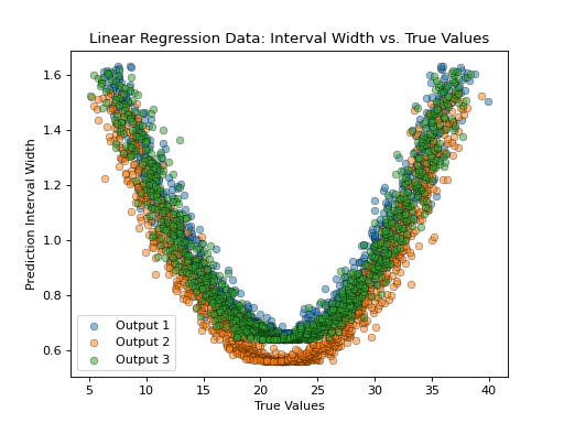
tfmelt.utils.visualization.plot_interval_width_vs_value(y_true, y_pred, y_std, ax, dataset_name, colors: List | None = ['#1f77b4', '#ff7f0e', '#2ca02c', '#d62728', '#9467bd', '#8c564b', '#e377c2', '#7f7f7f', '#bcbd22', '#17becf'], normalize: bool | None = False, use_pred: bool | None = False)

Plot the prediction interval width against the true or predicted values.

Parameters:

• y_true (array-like) – Actual values.

• y_pred (array-like) – Predicted values.

• y_std (array-like) – Standard deviation of predictions.

• ax – Matplotlib axes object.

• dataset_name (str) – Name of the dataset for labeling.

• colors (list, optional) – List of colors for the plot. Defaults to the default color cycle.

• normalize (bool, optional) – Whether to normalize the interval width by the range of the true values. Defaults to False.

• use_pred (bool, optional) – Whether to use predicted or true values on the x-axis. Defaults to False.

(Source code, png, hires.png, pdf)

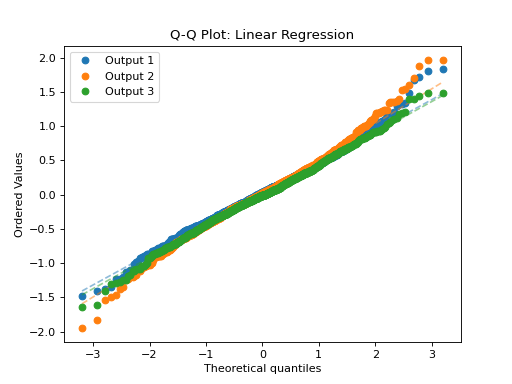
tfmelt.utils.visualization.plot_qq(ax, y_true, y_pred, y_std, dataset_name, colors: List | None = ['#1f77b4', '#ff7f0e', '#2ca02c', '#d62728', '#9467bd', '#8c564b', '#e377c2', '#7f7f7f', '#bcbd22', '#17becf'])

Plot Quantile-Quantile (Q-Q) plot using scipy.stats.probplot.

Parameters:

• ax – Matplotlib axes object.

• y_true (array-like) – Actual values.

• y_pred (array-like) – Predicted values.

• y_std (array-like) – Standard deviation of predictions.

• dataset_name (str) – Name of the dataset for labeling.

• colors (list, optional) – List of colors for the plot.

(Source code, png, hires.png, pdf)

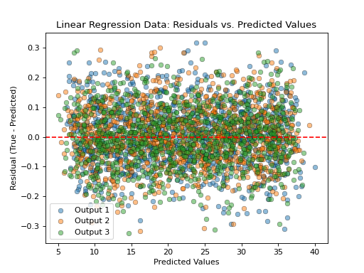
tfmelt.utils.visualization.plot_residuals_vs_value(y_true, y_pred, ax, dataset_name, colors: List | None = ['#1f77b4', '#ff7f0e', '#2ca02c', '#d62728', '#9467bd', '#8c564b', '#e377c2', '#7f7f7f', '#bcbd22', '#17becf'], use_pred: bool | None = True)

Plot the residuals (true - predicted) against the true or predicted values.

Parameters:

• y_true (array-like) – Actual values.

• y_pred (array-like) – Predicted values.

• ax – Matplotlib axes object.

• dataset_name (str) – Name of the dataset for labeling.

• colors (list, optional) – List of colors for the plot. Defaults to the default color cycle.

• use_pred (bool, optional) – Whether to use predicted or true values on the x-axis. Defaults to True.

(Source code, png, hires.png, pdf)

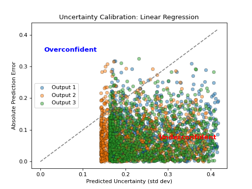
tfmelt.utils.visualization.plot_uncertainty_calibration(ax, y_true, y_pred, y_std, dataset_name, colors: List | None = ['#1f77b4', '#ff7f0e', '#2ca02c', '#d62728', '#9467bd', '#8c564b', '#e377c2', '#7f7f7f', '#bcbd22', '#17becf'])

Plot Uncertainty Calibration. This plot shows the absolute prediction error against the predicted uncertainty. The dashed line represents perfect calibration.

Parameters:

• ax – Matplotlib axes object.

• y_true (array-like) – Actual values.

• y_pred (array-like) – Predicted values.

• y_std (array-like) – Standard deviation of predictions.

• dataset_name (str) – Name of the dataset for labeling.

• colors (list) – List of colors for the plot.

(Source code, png, hires.png, pdf)

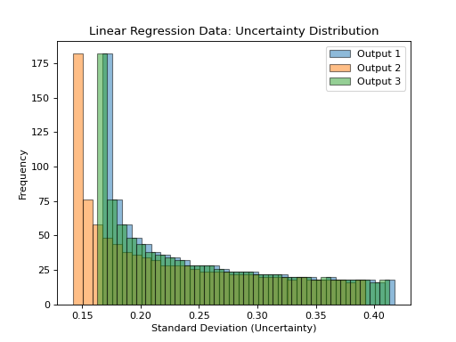
tfmelt.utils.visualization.plot_uncertainty_distribution(y_std, ax, dataset_name, colors: List | None = ['#1f77b4', '#ff7f0e', '#2ca02c', '#d62728', '#9467bd', '#8c564b', '#e377c2', '#7f7f7f', '#bcbd22', '#17becf'])

Plot the distribution of uncertainty (standard deviation) values.

Parameters:

• y_std (array-like) – Standard deviation of predictions.

• ax – Matplotlib axes object.

• dataset_name (str) – Name of the dataset for labeling.

• colors (list, optional) – List of colors for the plot. Defaults to the default color cycle.

(Source code, png, hires.png, pdf)

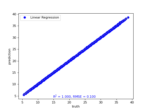
tfmelt.utils.visualization.point_cloud_plot(ax, y_real, y_pred, r_squared, rmse, label: str | None = None, marker: str | None = 'o', color: str | None = 'blue', text_pos: tuple | None = (0.3, 0.01))

Create a point cloud plot on the given axes.

Parameters:

• ax – Matplotlib axes object.

• y_real (array-like) – Actual values.

• y_pred (array-like) – Predicted values.

• r_squared (float) – R-squared value.

• rmse (float) – RMSE value.

• label (str, optional) – Label for the plot. Defaults to None.

• marker (str, optional) – Marker style. Defaults to “o”.

• color (str, optional) – Marker color. Defaults to “blue”.

• text_pos (tuple, optional) – Position for the RMSE text annotation (x, y). Defaults to (0.3, 0.01).

(Source code, png, hires.png, pdf)

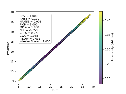
tfmelt.utils.visualization.point_cloud_plot_with_uncertainty(ax, y_real, y_pred, y_std, text_pos: tuple | None = (0.05, 0.95), metrics_to_display: List[str] | None = None)

Create a point cloud plot with uncertainty on the given axes.

Parameters:

• ax – Matplotlib axes object.

• y_real (array-like) – Actual values.

• y_pred (array-like) – Predicted values.

• y_std (array-like) – Standard deviation of predictions.

• text_pos (tuple, optional) – Position for the text annotation (x, y). Defaults to (0.05, 0.95).

• metrics_to_display (list of str, optional) – List of metrics to display in the text annotation. If None, all metrics in compute_metrics() are show. Defaults to None.

(Source code, png, hires.png, pdf)

tfmelt.utils.visualization.plot_history(history, metrics: List | None = ['loss'], plot_log: bool | None = False, savename: str | None = None)

Plot training history for specified metrics and optionally save the plot.

Parameters:

• history – History object from model training.

• metrics (list of str) – List of metrics to plot. Defaults to [“loss”].

• plot_log (bool) – Whether to include a logarithmic scale subplot. Defaults to False.

• savename (str) – Full path to save the plot image. If None, the plot will not be saved. Defaults to None.

tfmelt.utils.visualization.plot_predictions(pred_train, y_train_real, pred_val, y_val_real, pred_test, y_test_real, output_indices: List[int] | None = None, max_targets: int | None = 3, savename: str | None = None)

Plot predictions for specified output indices.

Parameters:

• pred_train (array-like) – Predicted training values.

• y_train_real (array-like) – Actual training values.

• pred_val (array-like) – Predicted validation values.

• y_val_real (array-like) – Actual validation values.

• pred_test (array-like) – Predicted test values.

• y_test_real (array-like) – Actual test values.

• output_indices (list of int, optional) – List of output indices to plot. Defaults to None.

• max_targets (int, optional) – Maximum number of targets to plot. Defaults to 3.

• savename (str, optional) – Full path to save the plot image. If None, the plot will not be saved. Defaults to None.

tfmelt.utils.visualization.plot_predictions_with_uncertainty(mean_train, std_train, y_train_real, mean_val, std_val, y_val_real, mean_test, std_test, y_test_real, metrics_to_display: List[str] | None = None, savename: str | None = None)

Plot predictions with uncertainty for training, validation, and test data.

Parameters:

• mean_train (array-like) – Training data.

• std_train (array-like) – Training data.

• y_train_real (array-like) – Training data.

• mean_val (array-like) – Validation data.

• std_val (array-like) – Validation data.

• y_val_real (array-like) – Validation data.

• mean_test (array-like) – Test data.

• std_test (array-like) – Test data.

• y_test_real (array-like) – Test data.

• metrics_to_display (list of str, optional) – List of metrics to display in the text annotation. If None, all metrics in compute_metrics() are show. Defaults to None.

• savename (str, optional) – Full path to save the plot image. If None, the plot will not be saved. Defaults to None.