OpenStreetMap example

In this example, we download a road network from OSM using the OSMNx package, and then process the result, resulting in a RouteE Compass network dataset.

requirements

To download an open street maps dataset, we'll need some extra dependnecies which are included with the conda distribution of this pacakge:

conda create -n routee-compass -c conda-forge python=3.11 nrel.routee.compass 

import osmnx as ox
import pandas as pd
import matplotlib.pyplot as plt

import json

from nrel.routee.compass.io import generate_compass_dataset
from nrel.routee.compass import CompassApp

# Try importing required packages to fail sooner if absent
try:
    import rasterio
    from osgeo import gdal
except:
    raise ImportError("Not all dependencies are installed")

---------------------------------------------------------------------------
ImportError                               Traceback (most recent call last)
Cell In[1], line 12
     11 try:
---> 12     import rasterio
     13     from osgeo import gdal

File /usr/share/miniconda/envs/test/lib/python3.11/site-packages/rasterio/__init__.py:28
     27 from rasterio._show_versions import show_versions
---> 28 from rasterio._version import gdal_version, get_geos_version, get_proj_version
     29 from rasterio.crs import CRS

ImportError: libpoppler.so.126: cannot open shared object file: No such file or directory

During handling of the above exception, another exception occurred:

ImportError                               Traceback (most recent call last)
Cell In[1], line 15
     13     from osgeo import gdal
     14 except:
---> 15     raise ImportError("Not all dependencies are installed")

ImportError: Not all dependencies are installed

Building RouteE Compass Dataset

Get OSM graph

First, we need to get an OSM graph that we can use to convert into the format RouteE Compass expects.

In this example we will load in a road network that covers Golden, Colorado as a small example, but this workflow will work with any osmnx graph (osmnx provides many graph download operations).

g = ox.graph_from_place("Denver, Colorado, USA", network_type="drive")  

Convert Graph to Compass Dataset

Now, we call the generate_compass_dataset function which will convert the osmnx graph into files that are compatible with RouteE Compass.

Note

In order to get the most accurate energy results from the routee-powertrain vehicle models, it's important to include road grade information since it plays a large factor in vehicle energy consumption (add_grade=True) That being said, adding grade can be a big lift computationally. In our case, we pull digital elevation model (DEM) raster files from USGS and then use osmnx to append elevation and grade to the graph. If the graph is large, this can take a while to download and could take up a lot of disk space. So, we recommend that you include grade information in your graph but want to be clear about the requirements for doing so.

generate_compass_dataset(g, output_directory="denver_co", add_grade=True)      

processing graph topology and speeds
adding grade information
processing vertices
processing edges
writing vertex files
writing edge files
writing edge attribute files
copying default configuration TOML files
copying RouteE Powertrain models

This will parse the OSM graph and write the RouteE Compass files into a new folder "denver_co/". If you take a look in this directory, you'll notice some .toml files like: osm_default_energy.toml. These are configurations for the compass application. Take a look here for more information about this file.

Running

Load Application

Now we can load the application from one of our config files. We'll pick osm_default_energy.toml for computing energy optimal routes.

app = CompassApp.from_config_file("denver_co/osm_default_energy.toml")  

uuid file: 100%|██████████| 16994/16994 [00:00<00:00, 6767659.50it/s]/s]

Queries

With our application loaded we can start computing routes by passing queries to the app. To demonstrate, we'll route between two locations in Denver, CO utilzing the grid search input plugin to run three separate searches.

The model_name is the vehicle we want to use for the route. If you look in the folder denver_co/models you'll see a collection of routee-powertrain models that can be used to compute the energy for your query.

The vehicle_state_variable_rates section defines rates to be applied to each component of the cost function. In this case we use the following costs:

• 0.655 dollars per mile

• 20 dollars per hour (or 0.333 dollars per minute)

• 3 dollars per gallon of gas

The grid_search section defines our test cases. Here, we have three cases: [least_time, least_energy, least_cost].
In the least_time and least_energy cases, we zero out all other variable contributions using the state_variable_coefficients which always get applied to each cost componenet. In the least_cost case, we allow each cost component to contribute equally and the algorithm will minimize the resulting cost from all components being added together (after getting multiplied by the appropriate vehicle_state_variable_rate.

query = [
    {
        "origin_x": -104.969307,
        "origin_y": 39.779021,
        "destination_x": -104.975360,
        "destination_y": 39.693005,
        "model_name": "2016_TOYOTA_Camry_4cyl_2WD",
        "vehicle_rates": {
            "distance": {"type": "factor", "factor": 0.655},
            "time": {"type": "factor", "factor": 0.33},
            "energy_liquid": {"type": "factor", "factor": 3.0},            
        },
        "grid_search": {
            "test_cases": [
              {
                "name": "least_time",
                "weights": {
                  "distance": 0,
                  "time": 1,
                  "energy_liquid": 0
                }
              },
              {
                "name": "least_energy",
                "weights": {
                  "distance": 0,
                  "time": 0,
                  "energy_liquid": 1
                }
              },
              {
                "name": "least_cost",
                "weights": {
                  "distance": 1,
                  "time": 1,
                  "energy_liquid": 1
                }
              }
            ]
          }    
    },
]

Now, let's pass the query to the application.

Note

A query can be a single object, or, a list of objects. If the input is a list of objects, the application will run these queries in parallel over the number of threads defined in the config file under the paralellism key (defaults to 2).

results = app.run(query)

search: 100%|██████████| 3/3 [00:00<00:00, 69.66it/s]4.43it/s]

Analysis

The application returns the results as a list of python dictionaries. Since we used the grid search to specify three separate searches, we should get three results back:

for r in results:
    error = r.get("error")
    if error is not None:
        print(f"request had error: {error}")

assert len(results)==3, f"expected 3 results, found {len(results)}"

Traversal and Cost Summaries

Since we have the traversal output plugin activated by default, we can take a look at the summary for each result under the traversal_summary key.

def pretty_print(dict):
    print(json.dumps(dict, indent=4))
    
shortest_time_result = next(filter(lambda r: r["request"]["name"] == "least_time", results))
least_energy_result = next(filter(lambda r: r["request"]["name"] == "least_energy", results))
least_cost_result = next(filter(lambda r: r["request"]["name"] == "least_cost", results))

Summary of route result for distance, time, and energy:

pretty_print(shortest_time_result["route"]["traversal_summary"])

{
    "distance": 9.152878807061885,
    "energy_liquid": 0.32013055234991905,
    "time": 10.897048882084228
}

And, if we need to know the units and/or the initial conditions for the search, we can look at the state model

pretty_print(shortest_time_result["route"]["state_model"])

{
    "distance": {
        "distance_unit": "miles",
        "initial": 0.0
    },
    "energy_liquid": {
        "energy_unit": "gallons_gasoline",
        "initial": 0.0
    },
    "time": {
        "initial": 0.0,
        "time_unit": "minutes"
    }
}

The cost section shows the costs per unit assigned to the trip, in dollars.

This is based on the user assumptions assigned in the configuration which can be overriden in the route request query.

pretty_print(shortest_time_result["route"]["cost"])

{
    "distance": 5.995135618625535,
    "energy_liquid": 0.9603916570497572,
    "time": 3.5960261310877955,
    "total_cost": 10.551553406763087
}

The cost_model section includes details for how these costs were calculated.

The user can set different state variable coefficients in the query that are weighted against the vehicle state variable rates.

The algorithm will rely on the weighted costs while the cost summary will show the final costs without weight coefficients applied.

pretty_print(shortest_time_result["route"]["cost_model"])

{
    "cost_aggregation": "sum",
    "distance": {
        "feature": "distance",
        "network_rate": {
            "type": "zero"
        },
        "vehicle_rate": {
            "factor": 0.655,
            "type": "factor"
        },
        "weight": 0.0
    },
    "energy_liquid": {
        "feature": "energy_liquid",
        "network_rate": {
            "type": "zero"
        },
        "vehicle_rate": {
            "factor": 3.0,
            "type": "factor"
        },
        "weight": 0.0
    },
    "time": {
        "feature": "time",
        "network_rate": {
            "type": "zero"
        },
        "vehicle_rate": {
            "factor": 0.33,
            "type": "factor"
        },
        "weight": 1.0
    }
}

Each response object contains this information. The least energy traversal and cost summary are below.

pretty_print(least_energy_result["route"]["traversal_summary"])
pretty_print(least_energy_result["route"]["cost"])

{
    "distance": 6.733433188572938,
    "energy_liquid": 0.2665045784952342,
    "time": 12.7747152207094
}
{
    "distance": 4.4103987385152745,
    "energy_liquid": 0.7995137354857025,
    "time": 4.215656022834102,
    "total_cost": 9.42556849683508
}

What becomes interesting is if we can compare our choices. Here's a quick comparison of the shortest time and least energy routes:

dist_diff = shortest_time_result["route"]["traversal_summary"]["distance"] - least_energy_result["route"]["traversal_summary"]["distance"]
time_diff = shortest_time_result["route"]["traversal_summary"]["time"] - least_energy_result["route"]["traversal_summary"]["time"]
enrg_diff = shortest_time_result["route"]["traversal_summary"]["energy_liquid"] - least_energy_result["route"]["traversal_summary"]["energy_liquid"]
cost_diff = shortest_time_result["route"]["cost"]["total_cost"] - least_energy_result["route"]["cost"]["total_cost"]
dist_unit = shortest_time_result["route"]["state_model"]["distance"]["distance_unit"]
time_unit = shortest_time_result["route"]["state_model"]["time"]["time_unit"]
enrg_unit = shortest_time_result["route"]["state_model"]["energy_liquid"]["energy_unit"]
print(f" - distance: {dist_diff:.2f} {dist_unit} further with time-optimal")
print(f" - time: {-time_diff:.2f} {time_unit} longer with energy-optimal")
print(f" - energy: {enrg_diff:.2f} {enrg_unit} more with time-optimal")
print(f" - cost: ${cost_diff:.2f} more with time-optimal")

 - distance: 2.42 miles further with time-optimal
 - time: 1.88 minutes longer with energy-optimal
 - energy: 0.05 gallons_gasoline more with time-optimal
 - cost: $1.13 more with time-optimal

In addition to the summary, the result also contains much more information. Here's a list of all the different sections that get returned:

def print_keys(d, indent=0):
    for k in sorted(d.keys()):
        print(f"{' '*indent} - {k}")
        if isinstance(d[k], dict):
            print_keys(d[k], indent+2)
print_keys(least_energy_result)

 - destination_vertex_uuid
 - iterations
 - origin_vertex_uuid
 - output_plugin_executed_time
 - request
   - destination_vertex
   - destination_x
   - destination_y
   - model_name
   - name
   - origin_vertex
   - origin_x
   - origin_y
   - query_weight_estimate
   - vehicle_rates
     - distance
       - factor
       - type
     - energy_liquid
       - factor
       - type
     - time
       - factor
       - type
   - weights
     - distance
     - energy_liquid
     - time
 - route
   - cost
     - distance
     - energy_liquid
     - time
     - total_cost
   - cost_model
     - cost_aggregation
     - distance
       - feature
       - network_rate
         - type
       - vehicle_rate
         - factor
         - type
       - weight
     - energy_liquid
       - feature
       - network_rate
         - type
       - vehicle_rate
         - factor
         - type
       - weight
     - time
       - feature
       - network_rate
         - type
       - vehicle_rate
         - factor
         - type
       - weight
   - path
     - features
     - type
   - state_model
     - distance
       - distance_unit
       - initial
     - energy_liquid
       - energy_unit
       - initial
     - time
       - initial
       - time_unit
   - traversal_summary
     - distance
     - energy_liquid
     - time
 - route_edges
 - search_executed_time
 - search_result_size_mib
 - search_runtime
 - tree_size_count

Plotting

We can also plot the results to see the difference between the two routes.

from nrel.routee.compass.plot import plot_route_folium, plot_routes_folium

We can use the plot_route_folium function to plot single routes, passing in the line_kwargs parameter to customize the folium linestring:

m = plot_route_folium(shortest_time_result, line_kwargs={"color": "red", "tooltip": "Shortest Time"})
m = plot_route_folium(least_energy_result, line_kwargs={"color": "green", "tooltip": "Least Energy"}, folium_map=m)
m = plot_route_folium(least_cost_result, line_kwargs={"color": "blue", "tooltip": "Least Cost"}, folium_map=m)
m

Make this Notebook Trusted to load map: File -> Trust Notebook

We can also use the plot_routes_folium function and pass in multiple results. The function will color the routes based on the value_fn which takes a single result as an argument. For example, we can tell it to color the routes based on the total energy usage.

folium_map = plot_routes_folium(results, value_fn=lambda r: r["route"]["traversal_summary"]["energy_liquid"], color_map="plasma")
folium_map

Make this Notebook Trusted to load map: File -> Trust Notebook

And the plot_routes_folium can also accept an existing folium_map parameter. Let's query our application with different origin and destination places:

query[0] = {
    **query[0],
    "origin_x": -105.081406,
    "origin_y": 39.667736,
    "destination_x": -104.95414,
    "destination_y": 39.65316,
}
new_results = app.run(query)

search: 100%|██████████| 3/3 [00:00<00:00, 64.03it/s]1.22it/s]

folium_map = plot_routes_folium(new_results, value_fn=lambda r: r["route"]["traversal_summary"]["energy_liquid"], color_map="plasma", folium_map=folium_map)
folium_map

Make this Notebook Trusted to load map: File -> Trust Notebook

Tradeoffs

Lastly, let's look at the tradeoffs for taking one route versus another.

First we'll gather some of the summary values into a dataframe:

c = []
for r in results:
    c.append({ 
        "scenario": r["request"]["name"],
        "time_minutes": r["route"]["traversal_summary"]["time"],
        "distance_miles": r["route"]["traversal_summary"]["distance"],
        "energy_gge": r["route"]["traversal_summary"]["energy_liquid"],
        "cost_dollars": r["route"]["cost"]["total_cost"],
    })

df = pd.DataFrame(c)
df

	scenario	time_minutes	distance_miles	energy_gge	cost_dollars
0	least_time	10.897049	9.152879	0.320131	10.551553
1	least_cost	13.158831	6.470756	0.280432	9.422056
2	least_energy	12.774715	6.733433	0.266505	9.425568

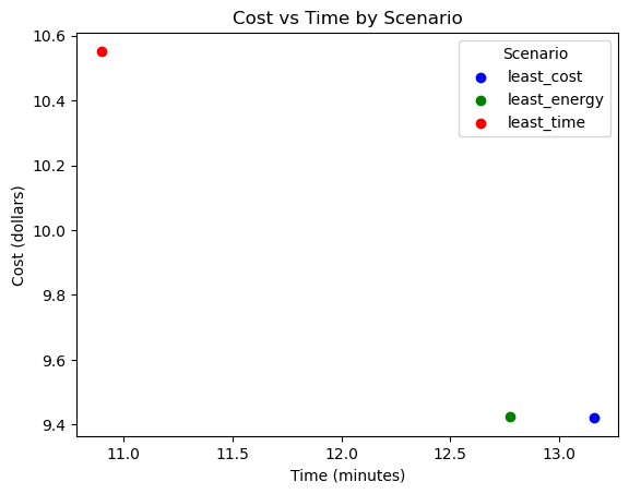
Now, let's look at the tradeoff between time and cost.

fig, ax = plt.subplots()
colors = {'least_time':'red', 'least_cost':'blue', 'least_energy':'green'}

for scenario, group in df.groupby('scenario'):
    ax.scatter(group['time_minutes'], group['cost_dollars'], color=colors[scenario], label=scenario)

ax.set_xlabel('Time (minutes)')
ax.set_ylabel('Cost (dollars)')
ax.legend(title='Scenario')
plt.title('Cost vs Time by Scenario')

Text(0.5, 1.0, 'Cost vs Time by Scenario')

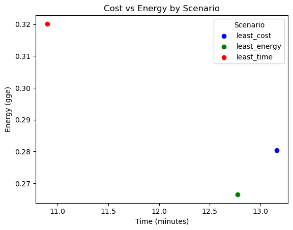
Next, let's look at the time versus energy tradeoff

fig, ax = plt.subplots()

for scenario, group in df.groupby('scenario'):
    ax.scatter(group['time_minutes'], group['energy_gge'], color=colors[scenario], label=scenario)

ax.set_xlabel('Time (minutes)')
ax.set_ylabel('Energy (gge)')
ax.legend(title='Scenario')
plt.title('Cost vs Energy by Scenario')

Text(0.5, 1.0, 'Cost vs Energy by Scenario')

Running Other Powertrain Types

RouteE Compass can execute search plans for internal combustion (ICE), plug-in hybrid (PHEV) and battery electric (BEV) powertrain types. Each of these powertrain types are represented by RouteE Powertrain models. To see all the models we can use you can take a look at the folder denver_co/models and then reference the traversal.vehicles section of the osm_default_energy.toml configuration file to see how they are integrated and what name is expected as the model_name parameter in the query. Note that you can also train your own RouteE Powertrain models. Take a look at this notebook for more details.

To demonstrate running other powertrain types, we'll use a BEV and a PHEV model and create queries for each powertrain type. In this case we'll select a 2017 Chevrolet Bolt and modify the query above to make it compatible with that vehicle. The only major changes to note is that we need to provide a weight and vehicle rate for energy_electric instead of energy_liquid. We can also specify the starting_soc_percent that represents the vehicles battery state of charge at the begining of the trip.

bev_query = [
    {
        "origin_x": -104.969307,
        "origin_y": 39.779021,
        "destination_x": -104.975360,
        "destination_y": 39.693005,
        "model_name": "2017_CHEVROLET_Bolt",
        "starting_soc_percent": 100,
        "vehicle_rates": {
            "distance": {"type": "factor", "factor": 0.655},
            "time": {"type": "factor", "factor": 0.33},
            "energy_electric": {"type": "factor", "factor": 0.5},            
        },
        "grid_search": {
            "test_cases": [
              {
                "name": "least_time",
                "weights": {
                  "distance": 0,
                  "time": 1,
                  "energy_electric": 0
                }
              },
              {
                "name": "least_energy",
                "weights": {
                  "distance": 0,
                  "time": 0,
                  "energy_electric": 1
                }
              },
              {
                "name": "least_cost",
                "weights": {
                  "distance": 1,
                  "time": 1,
                  "energy_electric": 1
                }
              }
            ]
          }    
    },
]

bev_result = app.run(bev_query)

search: 100%|██████████| 3/3 [00:00<00:00, 61.29it/s]4.12it/s]

Now we can take a look at the results. First let's take out the first result and look at the state model.

pretty_print(bev_result[0]["route"]["state_model"])

{
    "battery_state": {
        "format": {
            "floating_point": {
                "initial": 100.0
            }
        },
        "type": "soc",
        "unit": "percent"
    },
    "distance": {
        "distance_unit": "miles",
        "initial": 0.0
    },
    "energy_electric": {
        "energy_unit": "kilowatt_hours",
        "initial": 0.0
    },
    "time": {
        "initial": 0.0,
        "time_unit": "minutes"
    }
}

Here we see that we're tracking both energy (in kwh) and the battery state (in percent). If we then look at the traversal summary we see how much energy the vehicle consumed and we also note the state of the battery at the end of the route

pretty_print(bev_result[0]["route"]["traversal_summary"])

{
    "battery_state": 95.01694417725626,
    "distance": 9.152878807061885,
    "energy_electric": 2.989833493646233,
    "time": 10.897048882084228
}

Next we'll look at a PHEV powertrain type. In this query, everything will be similar to the battery electric vehicle but we'll be tracking both electrical energy and gasoline energy. By default, the PHEV will run using battery energy exclusively (starting at starting_soc_percent) and when the battery runs out, the vehicle will switch to it's hybrid mode, using primarily gasoline energy.

phev_query = [
    {
        "origin_x": -104.969307,
        "origin_y": 39.779021,
        "destination_x": -104.975360,
        "destination_y": 39.693005,
        "model_name": "2016_CHEVROLET_Volt",
        "starting_soc_percent": 100,
        "vehicle_rates": {
            "distance": {"type": "factor", "factor": 0.655},
            "time": {"type": "factor", "factor": 0.33},
            "energy_electric": {"type": "factor", "factor": 0.5},
            "energy_liquid": {"type": "factor", "factor": 3.0},   
        },
        "grid_search": {
            "test_cases": [
              {
                "name": "least_time",
                "weights": {
                  "distance": 0,
                  "time": 1,
                  "energy_electric": 0,
                  "energy_liquid": 0
                }
              },
              {
                "name": "least_energy",
                "weights": {
                  "distance": 0,
                  "time": 0,
                  "energy_electric": 1,
                  "energy_liquid": 1
                }
              },
              {
                "name": "least_cost",
                "weights": {
                  "distance": 1,
                  "time": 1,
                  "energy_electric": 1,
                  "energy_liquid": 1
                }
              }
            ]
          }    
    },
]

phev_results = app.run(phev_query)

search: 100%|██████████| 3/3 [00:00<00:00, 44.46it/s]1.88it/s]

pretty_print(phev_results[0]["route"]["state_model"])

{
    "battery_state": {
        "format": {
            "floating_point": {
                "initial": 100.0
            }
        },
        "type": "soc",
        "unit": "percent"
    },
    "distance": {
        "distance_unit": "miles",
        "initial": 0.0
    },
    "energy_electric": {
        "energy_unit": "kilowatt_hours",
        "initial": 0.0
    },
    "energy_liquid": {
        "energy_unit": "gallons_gasoline",
        "initial": 0.0
    },
    "time": {
        "initial": 0.0,
        "time_unit": "minutes"
    }
}

pretty_print(phev_results[0]["route"]["traversal_summary"])

{
    "battery_state": 78.14694106580795,
    "distance": 9.152878807061885,
    "energy_electric": 2.6223670721030534,
    "energy_liquid": 0.0,
    "time": 10.897048882084228
}

Note that we get back both electrical and gasoline energy values and in this case the route was short enough that the vehicle was able run on the battery exclusively.

At this point we could repeat all of the analysis above with the new results (plotting, tradeoffs, etc).