Hosting Capacity Analysis¶

This section shows how to conduct hosting capacity analysis using DISCO pipeline with snapshot and time-series models as inputs. This tutorial assumes there’s an existing snapshot-feeder-models directory generated from the transform-model command as below. The workflow below can also be applied to time-series-feeder-models.

1. Config Pipeline

Check the --help option for creating pipeline template.

$ disco create-pipeline template --help
Usage: disco create-pipeline template [OPTIONS] INPUTS

Create pipeline template file

Options:
-T, --task-name TEXT            The task name of the simulation/analysis
                                [required]
-P, --preconfigured             Whether inputs models are preconfigured
                                [default: False]
-s, --simulation-type [snapshot|time-series|upgrade]
                                Choose a DISCO simulation type  [default:
                                snapshot]
--with-loadshape / --no-with-loadshape
                                Indicate if loadshape file used for Snapshot
                                simulation.
--auto-select-time-points / --no-auto-select-time-points
                                Automatically select the time point based on
                                max PV-load ratio for snapshot simulations.
                                Only applicable if --with-loadshape.
                                [default: auto-select-time-points]
-d, --auto-select-time-points-search-duration-days INTEGER
                                Search duration in days. Only applicable
                                with --auto-select-time-points.  [default:
                                365]
-i, --impact-analysis           Enable impact analysis computations
                                [default: False]
-h, --hosting-capacity          Enable hosting capacity computations
                                [default: False]
-u, --upgrade-analysis          Enable upgrade cost computations  [default:
                                False]
-c, --cost-benefit              Enable cost benefit computations  [default:
                                False]
-p, --prescreen                 Enable PV penetration level prescreening
                                [default: False]
-t, --template-file TEXT        Output pipeline template file  [default:
                                pipeline-template.toml]
-r, --reports-filename TEXT     PyDSS report options. If None, use the
                                default for the simulation type.
-S, --enable-singularity        Add Singularity parameters and set the
                                config to run in a container.  [default:
                                False]
-C, --container PATH            Path to container
-D, --database PATH             The path of new or existing SQLite database
                                [default: results.sqlite]
-l, --local                     Run in local mode (non-HPC).  [default:
                                False]
--help                          Show this message and exit.

Given an output directory from transform-model, we use this command with --preconfigured option to create the template.

$ disco create-pipeline template -T SnapshotTask -s snapshot -h -P snapshot-feeder-models --with-loadshape

Note

For configuring a dynamic hosting capacity pipeline, use -s time-series

It creates pipeline-template.toml with configurable parameters of different sections. Update parameter values if needed. Then run

$ disco create-pipeline config pipeline-template.toml

This command creates a pipeline.json file containing two stages:

stage 1 - simulation
stage 2 - post-process

Accordingly, there will be an output directory for each stage,

output-stage1
output-stage2

2. Submit Pipeline

With a configured DISCO pipeline in pipeline.json the next step is to submit the pipeline with JADE:

$ jade pipeline submit pipeline.json -o output

What does each stage do?

In the simulation stage DISCO runs a power flow simulation for each job through PyDSS and stores per-job metrics.
In the post-process stage DISCO aggregates the metrics from each simulation job, calculates the hosting capacity, and then ingests results into a SQLite database.

3. Check Results

The post-process stage aggregates metrics in the following tables in output/output-stage1:

feeder_head_table.csv
feeder_losses_table.csv
metadata_table.csv
thermal_metrics_table.csv
voltage_metrics_table.csv

Each table contains metrics related to the snapshot or time-series simulation. DISCO computes hosting capacity results from these metrics and then writes them to the following files, also in output/output-stage1:

hosting_capacity_summary__<scenario_name>.json
hosting_capacity_overall__<scenario_name>.json

The scenario name will be scenario, pf1 and/or control_mode, depending on your simulation type and/or --with-loadshape option.

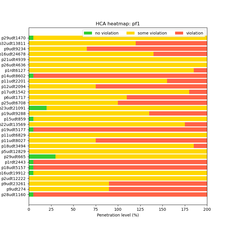
Note that DISCO also produces prototypical visualizations for hosting capacity automatically after each run:

hca__{scenario_name}.png

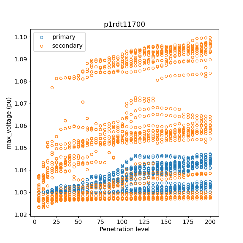
The voltage plot examples for the first feeder comparing pf1 vs. voltvar and comparing primary and secondary voltages:

max_voltage_pf1_voltvar.png
max_voltage_pri_sec.png

4. Results database

DISCO ingests the hosting capacity results and report metrics into a SQLite database named output/output-stage1/results.sqlite. You can use standard SQL to query data, and perform further analysis.

If you want to ingest the results into an existing database, please specify the absolute path of the database in pipeline.toml.

For sqlite query examples, please refer to the Jupyter notebook notebooks/db-query.ipynb in the source code repo.

If you would like to use the CLI tool sqlite3 directly, here are some examples. Note that in this case the database contains the results from a single task, and so the queries are not first pre-filtering the tables.

If you don’t already have sqlite3 installed, please refer to their website.

Run this command to start the CLI utility:

$ sqlite3 -table <path-to-db.sqlite>

Note

If your version of sqlite3 doesn’t support -table, use -header -column instead.

View DISCO’s hosting capacity results for all feeders.

sqlite> SELECT * from hosting_capacity WHERE hc_type = 'overall';

View voltage violations for one feeder and scenario.

sqlite> SELECT feeder, scenario, sample, penetration_level, node_type, min_voltage, max_voltage
        FROM voltage_metrics
        WHERE (max_voltage > 1.05 or min_voltage < 0.95)
        AND scenario = 'pf1'
        AND feeder = 'p19udt14287';

View the min and max voltages for each penetration_level (across samples) for one feeder.

sqlite> SELECT feeder, sample, penetration_level
        ,MIN(min_voltage) as min_voltage_overall
        ,MAX(max_voltage) as max_voltage_overall
        ,MAX(num_nodes_any_outside_ansi_b) as num_nodes_any_outside_ansi_b_overall
        ,MAX(num_time_points_with_ansi_b_violations) as num_time_points_with_ansi_b_violations_overall
        FROM voltage_metrics
        WHERE scenario = 'pf1'
        AND feeder = 'p19udt14287'
        GROUP BY feeder, penetration_level;

View the max thermal loadings for each penetration_level (across samples) for one feeder.

sqlite> SELECT feeder, sample, penetration_level
        ,MAX(line_max_instantaneous_loading_pct) as line_max_inst
        ,MAX(line_max_moving_average_loading_pct) as line_max_mavg
        ,MAX(line_num_time_points_with_instantaneous_violations) as line_num_inst
        ,MAX(line_num_time_points_with_moving_average_violations) as line_num_mavg
        ,MAX(transformer_max_instantaneous_loading_pct) as xfmr_max_inst
        ,MAX(transformer_max_moving_average_loading_pct) as xfmr_max_mavg
        ,MAX(transformer_num_time_points_with_instantaneous_violations) as xfmr_num_inst
        ,MAX(transformer_num_time_points_with_moving_average_violations) as xfmr_num_mavg
        FROM thermal_metrics
        WHERE scenario = 'pf1'
        AND feeder = 'p19udt14287'
        GROUP BY feeder, penetration_level;