Analysis Example

Multiple Objectives for Residential PV.

Import packages.

import os
import sys
sys.path.insert(0, os.path.abspath("../src"))

import numpy             as np
import matplotlib.pyplot as pl
import pandas            as pd
import seaborn           as sb
import tyche             as ty

from copy            import deepcopy
from IPython.display import Image

Load data.

The data should be stored in a set of comma-separated value files in a sub-directory of the technology folder, as shown in the directory structure diagram (Fig. 1)

designs = ty.Designs("data/pv_residential_simple")

investments = ty.Investments("data/pv_residential_simple")

Compile the production and metric functions for each technology in the dataset.

designs.compile()

Examine the data.

The functions table specifies where the Python code for each technology resides.

designs.functions

	Style	Module	Capital	Fixed	Production	Metrics	Notes
Technology
Residential PV	numpy	pv_residential_simple	capital_cost	fixed_cost	production	metrics

Right now, only the style numpy is supported.

The indices table defines the subscripts for variables.

designs.indices

			Offset	Description	Notes
Technology	Type	Index
Residential PV	Capital	BoS	2	balance of system
		Inverter	1	system inverters
		Module	0	system module
	Fixed	System	0	whole system
	Input	NaN	0	no inputs
	Metric	GHG	2	reduction in GHGs
		LCOE	0	reduction in levelized cost of energy
		Labor	1	increase in spending on wages
	Output	Electricity	0	electricity generated

The designs table contains the cost, input, efficiency, and price data resulting from a Tranche.

designs.designs

				Value	Units	Notes
Technology	Tranche	Variable	Index
Residential PV	2015 Actual	Input	NaN	0	1	no inputs
		Input efficiency	NaN	1	1	no inputs
		Input price	NaN	0	1	no inputs
		Lifetime	BoS	1	system-lifetime	per-lifetime computations
			Inverter	1	system-lifetime	per-lifetime computations
	...	...	...	...	...	...
	Module Slow Progress	Lifetime	Inverter	1	system-lifetime	per-lifetime computations
			Module	1	system-lifetime	per-lifetime computations
		Output efficiency	Electricity	1	W/W	see parameter table for individual efficiencies
		Output price	Electricity	0	$/kWh	not tracking electricity price
		Scale	NaN	1	system/system	no scaling

90 rows × 3 columns

The parameters table contains additional techno-economic parameters for each technology.

designs.parameters

			Offset	Value	Units	Notes
Technology	Tranche	Parameter
Residential PV	2015 Actual	Customer Acquisition	19	st.triang(0.5, loc=2000, scale=0.2)	$/system	BCA
		DC-to-AC Ratio	15	st.triang(0.5, loc=1.4, scale=0.00014)	1	IDC
		Direct Labor	17	st.triang(0.5, loc=2000, scale=0.2)	$/system	BLR
		Discount Rate	0	0.07	1/year	DR
		Hardware Capital	16	st.triang(0.5, loc=80, scale=0.008)	$/m^2	BCC
	...	...	...	...	...	...
	Module Slow Progress	Module Lifetime	4	st.triang(0.5, loc=26, scale=1)	yr	MLT
		Module O&M Fixed	7	st.triang(0.5, loc=19, scale=0.5)	$/kWyr	MOM
		Module Soiling Loss	10	st.triang(0.5, loc=0.05, scale=10E-06)	1	MSL
		Permitting	18	st.triang(0.5, loc=600, scale=0.06)	$/system	BPR
		System Size	2	36	m^2	SSZ

210 rows × 4 columns

The results table specifies the units of measure for results of computations.

designs.results

			Units	Notes
Technology	Variable	Index
Residential PV	Cost	Cost	$/system
	Metric	GHG	ΔgCO2e/system
		LCOE	Δ$/kWh
		Labor	Δ$/system
	Output	Electricity	kWh

The tranches table specifies multually exclusive possibilities for investments: only one Tranch may be selected for each Category.

investments.tranches

			Amount	Notes
Category	Tranche
BoS R&D	BoS High R&D	BoS Fast Progress	900000.0
	BoS Low R&D	BoS Slow Progress	300000.0
	BoS Medium R&D	BoS Moderate Progress	600000.0
Inverter R&D	Inverter High R&D	Inverter Fast Progress	3000000.0
	Inverter Low R&D	Inverter Slow Progress	1000000.0
	Inverter Medium R&D	Inverter Moderate Progress	2000000.0
Module R&D	Module High R&D	Module Fast Progress	4500000.0
	Module Low R&D	Module Slow Progress	1500000.0
	Module Medium R&D	Module Moderate Progress	3000000.0

The investments table bundles a consistent set of tranches (one per category) into an overall investment.

investments.investments

			Notes
Investment	Category	Tranche
High R&D	BoS R&D	BoS High R&D
	Inverter R&D	Inverter High R&D
	Module R&D	Module High R&D
Low R&D	BoS R&D	BoS Low R&D
	Inverter R&D	Inverter Low R&D
	Module R&D	Module Low R&D
Medium R&D	BoS R&D	BoS Medium R&D
	Inverter R&D	Inverter Medium R&D
	Module R&D	Module Medium R&D

Evaluate the Tranches in the dataset.

tranche_results = designs.evaluate_tranches(sample_count=50)

tranche_results.xs(1, level="Sample", drop_level=False)

					Value	Units
Technology	Tranche	Sample	Variable	Index
Residential PV	2015 Actual	1	Cost	Cost	19541.835826	$/system
			Metric	GHG	-0.001761	ΔgCO2e/system
				LCOE	-0.000019	Δ$/kWh
				Labor	-0.001281	Δ$/system
			Output	Electricity	184107.032791	kWh
	BoS Fast Progress	1	Cost	Cost	17524.525245	$/system
			Metric	GHG	-0.004254	ΔgCO2e/system
				LCOE	0.010936	Δ$/kWh
				Labor	-545.200985	Δ$/system
			Output	Electricity	184101.481909	kWh
	BoS Moderate Progress	1	Cost	Cost	17960.467902	$/system
			Metric	GHG	-0.001253	ΔgCO2e/system
				LCOE	0.008571	Δ$/kWh
				Labor	-331.852654	Δ$/system
			Output	Electricity	184108.162865	kWh
	BoS Slow Progress	1	Cost	Cost	19022.884313	$/system
			Metric	GHG	0.000327	ΔgCO2e/system
				LCOE	0.002802	Δ$/kWh
				Labor	-148.230849	Δ$/system
			Output	Electricity	184111.682213	kWh
	Inverter Fast Progress	1	Cost	Cost	18059.997438	$/system
			Metric	GHG	2.601021	ΔgCO2e/system
				LCOE	0.011024	Δ$/kWh
				Labor	-0.031111	Δ$/system
			Output	Electricity	189903.145647	kWh
	Inverter Moderate Progress	1	Cost	Cost	18713.047656	$/system
			Metric	GHG	2.537671	ΔgCO2e/system
				LCOE	0.007512	Δ$/kWh
				Labor	-0.034240	Δ$/system
			Output	Electricity	189762.072909	kWh
	Inverter Slow Progress	1	Cost	Cost	19224.862899	$/system
			Metric	GHG	2.435100	ΔgCO2e/system
				LCOE	0.004693	Δ$/kWh
				Labor	0.056486	Δ$/system
			Output	Electricity	189533.659025	kWh
	Module Fast Progress	1	Cost	Cost	18935.973204	$/system
			Metric	GHG	51.490235	ΔgCO2e/system
				LCOE	0.042746	Δ$/kWh
				Labor	0.013583	Δ$/system
			Output	Electricity	298774.134685	kWh
	Module Moderate Progress	1	Cost	Cost	18952.058689	$/system
			Metric	GHG	41.216046	ΔgCO2e/system
				LCOE	0.037432	Δ$/kWh
				Labor	0.029792	Δ$/system
			Output	Electricity	275894.626758	kWh
	Module Slow Progress	1	Cost	Cost	19656.198525	$/system
			Metric	GHG	14.794693	ΔgCO2e/system
				LCOE	0.015567	Δ$/kWh
				Labor	-0.007250	Δ$/system
			Output	Electricity	217057.134731	kWh

Save results.

tranche_results.to_csv("output/pv_residential_simple/example-analysis.csv")

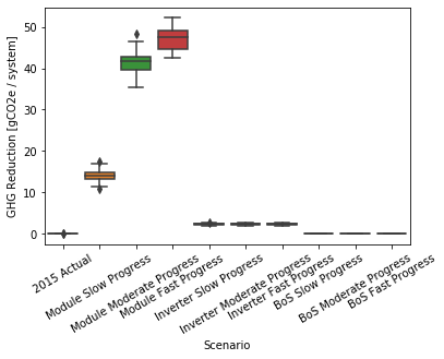
Plot GHG metric.

g = sb.boxplot(
    x="Tranche",
    y="Value",
    data=tranche_results.xs(
        ["Metric", "GHG"],
        level=["Variable", "Index"]
    ).reset_index()[["Tranche", "Value"]],
    order=[
        "2015 Actual"              ,
        "Module Slow Progress"      ,
        "Module Moderate Progress"  ,
        "Module Fast Progress"      ,
        "Inverter Slow Progress"    ,
        "Inverter Moderate Progress",
        "Inverter Fast Progress"    ,
        "BoS Slow Progress"         ,
        "BoS Moderate Progress"     ,
        "BoS Fast Progress"         ,
    ]
)
g.set(ylabel="GHG Reduction [gCO2e / system]")
g.set_xticklabels(g.get_xticklabels(), rotation=30);

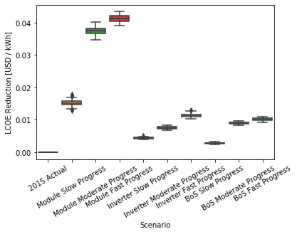
Plot LCOE metric.

g = sb.boxplot(
    x="Tranche",
    y="Value",
    data=tranche_results.xs(
        ["Metric", "LCOE"],
        level=["Variable", "Index"]
    ).reset_index()[["Tranche", "Value"]],
    order=[
        "2015 Actual"              ,
        "Module Slow Progress"      ,
        "Module Moderate Progress"  ,
        "Module Fast Progress"      ,
        "Inverter Slow Progress"    ,
        "Inverter Moderate Progress",
        "Inverter Fast Progress"    ,
        "BoS Slow Progress"         ,
        "BoS Moderate Progress"     ,
        "BoS Fast Progress"         ,
    ]
)
g.set(ylabel="LCOE Reduction [USD / kWh]")
g.set_xticklabels(g.get_xticklabels(), rotation=30);

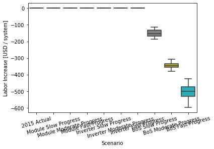
Plot labor metric.

g = sb.boxplot(
    x="Tranche",
    y="Value",
    data=tranche_results.xs(
        ["Metric", "Labor"],
        level=["Variable", "Index"]
    ).reset_index()[["Tranche", "Value"]],
    order=[
        "2015 Actual"              ,
        "Module Slow Progress"      ,
        "Module Moderate Progress"  ,
        "Module Fast Progress"      ,
        "Inverter Slow Progress"    ,
        "Inverter Moderate Progress",
        "Inverter Fast Progress"    ,
        "BoS Slow Progress"         ,
        "BoS Moderate Progress"     ,
        "BoS Fast Progress"         ,
    ]
)
g.set(ylabel="Labor Increase [USD / system]")
g.set_xticklabels(g.get_xticklabels(), rotation=15);

Evaluate the investments in the dataset.

investment_results = investments.evaluate_investments(designs, sample_count=50)

Costs of investments.

investment_results.amounts

	Amount
Investment
High R&D	8400000.0
Low R&D	2800000.0
Medium R&D	5600000.0

Benefits of investments.

investment_results.metrics.xs(1, level="Sample", drop_level=False)

							Value	Units
Investment	Category	Tranche	Sample	Technology	Index
High R&D	BoS R&D	BoS High R&D	BoS Fast Progress	1	Residential PV	GHG	0.001646	ΔgCO2e/system
						LCOE	0.009871	Δ$/kWh
						Labor	-484.675917	Δ$/system
Medium R&D	BoS R&D	BoS Medium R&D	BoS Moderate Progress	1	Residential PV	GHG	-0.005431	ΔgCO2e/system
						LCOE	0.009181	Δ$/kWh
						Labor	-350.111301	Δ$/system
Low R&D	BoS R&D	BoS Low R&D	BoS Slow Progress	1	Residential PV	GHG	-0.000623	ΔgCO2e/system
						LCOE	0.002863	Δ$/kWh
						Labor	-165.967402	Δ$/system
High R&D	Inverter R&D	Inverter High R&D	Inverter Fast Progress	1	Residential PV	GHG	2.366737	ΔgCO2e/system
						LCOE	0.011084	Δ$/kWh
						Labor	0.034014	Δ$/system
Medium R&D	Inverter R&D	Inverter Medium R&D	Inverter Moderate Progress	1	Residential PV	GHG	2.385654	ΔgCO2e/system
						LCOE	0.007551	Δ$/kWh
						Labor	0.016533	Δ$/system
Low R&D	Inverter R&D	Inverter Low R&D	Inverter Slow Progress	1	Residential PV	GHG	2.562178	ΔgCO2e/system
						LCOE	0.004598	Δ$/kWh
						Labor	0.081408	Δ$/system
High R&D	Module R&D	Module High R&D	Module Fast Progress	1	Residential PV	GHG	50.680545	ΔgCO2e/system
						LCOE	0.043544	Δ$/kWh
						Labor	-0.014162	Δ$/system
Medium R&D	Module R&D	Module Medium R&D	Module Moderate Progress	1	Residential PV	GHG	41.065128	ΔgCO2e/system
						LCOE	0.037053	Δ$/kWh
						Labor	-0.010921	Δ$/system
Low R&D	Module R&D	Module Low R&D	Module Slow Progress	1	Residential PV	GHG	12.916316	ΔgCO2e/system
						LCOE	0.013848	Δ$/kWh
						Labor	0.057653	Δ$/system

investment_results.summary.xs(1, level="Sample", drop_level=False)

			Value	Units
Investment	Sample	Index
High R&D	1	GHG	53.048928	ΔgCO2e/system
		LCOE	0.064500	Δ$/kWh
		Labor	-484.656066	Δ$/system
Medium R&D	1	GHG	43.445350	ΔgCO2e/system
		LCOE	0.053785	Δ$/kWh
		Labor	-350.105690	Δ$/system
Low R&D	1	GHG	15.477872	ΔgCO2e/system
		LCOE	0.021309	Δ$/kWh
		Labor	-165.828341	Δ$/system

Save results.

investment_results.amounts.to_csv("output/pv_residential_simple/example-investment-amounts.csv")

investment_results.metrics.to_csv("output/pv_residential_simple/example-investment-metrics.csv")

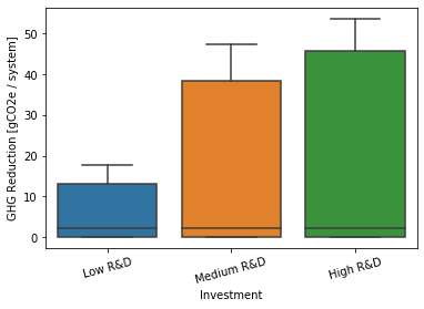
Plot GHG metric.

g = sb.boxplot(
    x="Investment",
    y="Value",
    data=investment_results.metrics.xs(
        "GHG",
        level="Index"
    ).reset_index()[["Investment", "Value"]],
    order=[
        "Low R&D"   ,
        "Medium R&D",
        "High R&D"  ,
    ]
)
g.set(ylabel="GHG Reduction [gCO2e / system]")
g.set_xticklabels(g.get_xticklabels(), rotation=15);

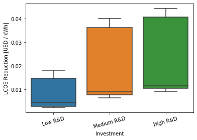
Plot LCOE metric.

g = sb.boxplot(
    x="Investment",
    y="Value",
    data=investment_results.metrics.xs(
        "LCOE",
        level="Index"
    ).reset_index()[["Investment", "Value"]],
    order=[
        "Low R&D"   ,
        "Medium R&D",
        "High R&D"  ,
    ]
)
g.set(ylabel="LCOE Reduction [USD / kWh]")
g.set_xticklabels(g.get_xticklabels(), rotation=15);

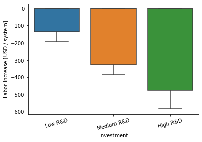
Plot labor metric.

g = sb.boxplot(
    x="Investment",
    y="Value",
    data=investment_results.metrics.xs(
        "Labor",
        level="Index"
    ).reset_index()[["Investment", "Value"]],
    order=[
        "Low R&D"   ,
        "Medium R&D",
        "High R&D"  ,
    ]
)
g.set(ylabel="Labor Increase [USD / system]")
g.set_xticklabels(g.get_xticklabels(), rotation=15);

Multi-objective decision analysis.

Compute costs and metrics for tranches.

Tranches are atomic units for building investment portfolios. Evaluate all of the tranches, so we can assemble them into investments (portfolios).

tranche_results = investments.evaluate_tranches(designs, sample_count=50)

Display the cost of each tranche.

tranche_results.amounts

		Amount
Category	Tranche
BoS R&D	BoS High R&D	900000.0
	BoS Low R&D	300000.0
	BoS Medium R&D	600000.0
Inverter R&D	Inverter High R&D	3000000.0
	Inverter Low R&D	1000000.0
	Inverter Medium R&D	2000000.0
Module R&D	Module High R&D	4500000.0
	Module Low R&D	1500000.0
	Module Medium R&D	3000000.0

Display the metrics for each tranche.

tranche_results.summary

				Value	Units
Category	Tranche	Sample	Index
BoS R&D	BoS High R&D	1	GHG	-0.004062	ΔgCO2e/system
			LCOE	0.009967	Δ$/kWh
			Labor	-490.859314	Δ$/system
		2	GHG	0.001960	ΔgCO2e/system
			LCOE	0.010154	Δ$/kWh
...	...	...	...	...	...
Module R&D	Module Low R&D	49	LCOE	0.016198	Δ$/kWh
			Labor	0.039788	Δ$/system
		50	GHG	13.654483	ΔgCO2e/system
			LCOE	0.014910	Δ$/kWh
			Labor	-0.015539	Δ$/system

1350 rows × 2 columns

Save the results.

tranche_results.amounts.to_csv("output/pv_residential_simple/example-tranche-amounts.csv")
tranche_results.summary.to_csv("output/pv_residential_simple/example-tranche-summary.csv")

Fit a response surface to the results.

The response surface interpolates between the discrete set of cases provided in the expert elicitation. This allows us to study funding levels intermediate between the pre-defined Tranches.

evaluator = ty.Evaluator(investments.tranches, tranche_results.summary)

Here are the categories of investment and the maximum amount that could be invested in each:

evaluator.max_amount

	Amount
Category
BoS R&D	900000.0
Inverter R&D	3000000.0
Module R&D	4500000.0

Here are the metrics and their units of measure:

evaluator.units

	Units
Index
GHG	ΔgCO2e/system
LCOE	Δ$/kWh
Labor	Δ$/system

Example interpolation.

Let’s evaluate the case where each category is invested in at half of its maximum amount.

example_investments = evaluator.max_amount / 2
example_investments

	Amount
Category
BoS R&D	450000.0
Inverter R&D	1500000.0
Module R&D	2250000.0

evaluator.evaluate(example_investments)

Category    Index  Sample
BoS R&D     GHG    1         -0.0010586097518157094
                   2          7.493162517135921e-05
                   3           0.001253893601450784
                   4           -0.00398626797827717
                   5          -0.005572343870333896
                                      ...
Module R&D  Labor  46          0.014371009324918305
                   47          0.011128728287076228
                   48         0.0039832773605894545
                   49          0.006026680267950724
                   50          0.028844695933457842
Name: Value, Length: 450, dtype: object

Let’s evaluate the mean instead of outputing the whole distribution.

evaluator.evaluate_statistic(example_investments, np.mean)

Index
GHG       30.156830
LCOE       0.038160
Labor   -246.843027
Name: Value, dtype: float64

Here is the standard deviation:

evaluator.evaluate_statistic(example_investments, np.std)

Index
GHG       1.410956
LCOE      0.000850
Labor    16.070395
Name: Value, dtype: float64

A risk-averse decision maker might be interested in the 10% percentile:

evaluator.evaluate_statistic(example_investments, lambda x: np.quantile(x, 0.1))

Index
GHG       28.573627
LCOE       0.037140
Labor   -268.059699
Name: Value, dtype: float64

ε-Constraint multiobjective optimization

optimizer = ty.EpsilonConstraintOptimizer(evaluator)

In order to meaningfully map the decision space, we need to know the maximum values for each of the metrics.

metric_max = optimizer.max_metrics()
metric_max

GHG      49.429976
LCOE      0.062818
Labor     0.049555
Name: Value, dtype: float64

Example optimization.

Limit spending to $3M.

investment_max = 3e6

Require that the GHG reduction be at least 40 gCO2e/system and that the Labor wages not decrease.

metric_min = pd.Series([40, 0], name = "Value", index = ["GHG", "Labor"])
metric_min

GHG      40
Labor     0
Name: Value, dtype: int64

Compute the ε-constrained maximum for the LCOE.

optimum = optimizer.maximize(
    "LCOE"                       ,
    total_amount = investment_max,
    min_metric   = metric_min    ,
    statistic    = np.mean       ,
)
optimum.exit_message

'Optimization terminated successfully.'

Here are the optimal spending levels:

np.round(optimum.amounts)

Category
BoS R&D               0.0
Inverter R&D          0.0
Module R&D      3000000.0
Name: Amount, dtype: float64

Here are the three metrics at that optimum:

optimum.metrics

Index
GHG      41.627691
LCOE      0.037566
Labor     0.028691
Name: Value, dtype: float64

Thus, by putting all of the investment into Module R&D, we can expected to achieve a mean 3.75 ¢/kWh reduction in LCOE under the GHG and Labor constraints.

It turns out that there is no solution for these constraints if we evaluate the 10th percentile of the metrics, for a risk-averse decision maker.

optimum = optimizer.maximize(
    "LCOE"                       ,
    total_amount = investment_max,
    min_metric   = metric_min    ,
    statistic    = lambda x: np.quantile(x, 0.1),
)
optimum.exit_message

'Iteration limit exceeded'

Let’s try again, but with a less stringent set of constraints, only constraining GHG somewhat but not Labor at all.

optimum = optimizer.maximize(
    "LCOE"                                                         ,
    total_amount = investment_max                                  ,
    min_metric   = pd.Series([30], name = "Value", index = ["GHG"]),
    statistic    = lambda x: np.quantile(x, 0.1)                   ,
)
optimum.exit_message

'Optimization terminated successfully.'

np.round(optimum.amounts)

Category
BoS R&D               0.0
Inverter R&D          0.0
Module R&D      3000000.0
Name: Amount, dtype: float64

optimum.metrics

Index
GHG      39.046988
LCOE      0.036463
Labor    -0.019725
Name: Value, dtype: float64

Pareto surfaces.

Metrics constrained by total investment.

pareto_amounts = None
for investment_max in np.arange(1e6, 9e6, 0.5e6):
    metrics = optimizer.max_metrics(total_amount = investment_max)
    pareto_amounts = pd.DataFrame(
        [metrics.values]                                         ,
        columns = metrics.index.values                           ,
        index   = pd.Index([investment_max / 1e6], name = "Investment [M$]"),
    ).append(pareto_amounts)
pareto_amounts

	GHG	LCOE	Labor
Investment [M$]
8.5	49.429976	0.062818	0.049555
8.0	49.429976	0.061848	0.049555
7.5	49.429976	0.060635	0.049555
7.0	49.429976	0.059423	0.049555
6.5	49.429976	0.057592	0.049560
6.0	49.426992	0.055608	0.049545
5.5	49.424007	0.053976	0.049104
5.0	48.278589	0.052171	0.048930
4.5	47.133172	0.050431	0.047878
4.0	45.298011	0.048243	0.046810
3.5	43.462851	0.045006	0.042130
3.0	41.627691	0.037569	0.037450
2.5	32.453455	0.030129	0.032769
2.0	23.279219	0.023166	0.027886
1.5	14.104983	0.018081	0.023003
1.0	9.403322	0.010170	0.018119

sb.relplot(
    x         = "Investment [M$]",
    y         = "Value"          ,
    col       = "Metric"         ,
    kind      = "line"           ,
    facet_kws = {'sharey': False},
    data      = pareto_amounts.reset_index().melt(id_vars = "Investment [M$]", var_name = "Metric", value_name = "Value")
)

<seaborn.axisgrid.FacetGrid at 0x7f9da11752b0>

We see that the LCOE metric saturates more slowly than the GHG and Labor ones.

GHG vs LCOE, constrained by total investment.

investment_max = 3
pareto_ghg_lcoe = None
for lcoe_min in 0.95 * np.arange(0.5, 0.9, 0.05) * pareto_amounts.loc[investment_max, "LCOE"]:
    optimum = optimizer.maximize(
        "GHG",
        max_amount   = pd.Series([0.9e6, 3.0e6, 1.0e6], name = "Amount", index = ["BoS R&D", "Inverter R&D", "Module R&D"]),
        total_amount = investment_max * 1e6                                 ,
        min_metric   = pd.Series([lcoe_min], name = "Value", index = ["LCOE"]),
    )
    pareto_ghg_lcoe = pd.DataFrame(
        [[investment_max, lcoe_min, optimum.metrics["LCOE"], optimum.metrics["GHG"], optimum.exit_message]],
        columns = ["Investment [M$]", "LCOE (min)", "LCOE", "GHG", "Result"]                               ,
    ).append(pareto_ghg_lcoe)
pareto_ghg_lcoe = pareto_ghg_lcoe.set_index(["Investment [M$]", "LCOE (min)"])
pareto_ghg_lcoe

		LCOE	GHG	Result
Investment [M$]	LCOE (min)
3	0.030337	0.025037	11.691901	Positive directional derivative for linesearch
	0.028553	0.025037	11.691901	Positive directional derivative for linesearch
	0.026768	0.025037	11.691901	Positive directional derivative for linesearch
	0.024983	0.024983	11.692188	Optimization terminated successfully.
	0.023199	0.023199	11.693916	Optimization terminated successfully.
	0.021414	0.021414	11.694230	Optimization terminated successfully.
	0.019630	0.019630	11.694544	Optimization terminated successfully.
	0.017845	0.017845	11.699478	Optimization terminated successfully.

sb.relplot(
    x = "LCOE",
    y = "GHG",
    kind = "scatter",
    data = pareto_ghg_lcoe#[pareto_ghg_lcoe.Result == "Optimization terminated successfully."]
)

<seaborn.axisgrid.FacetGrid at 0x7f9da13ae630>

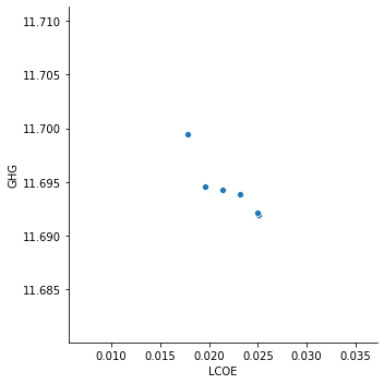
The three types of investment are too decoupled to make an interesting pareto frontier, and we also need a better solver if we want to push to lower right.

Run the interactive explorer for the decision space.

Make sure the the tk package is installed on your machine. Here is the Anaconda link: https://anaconda.org/anaconda/tk.

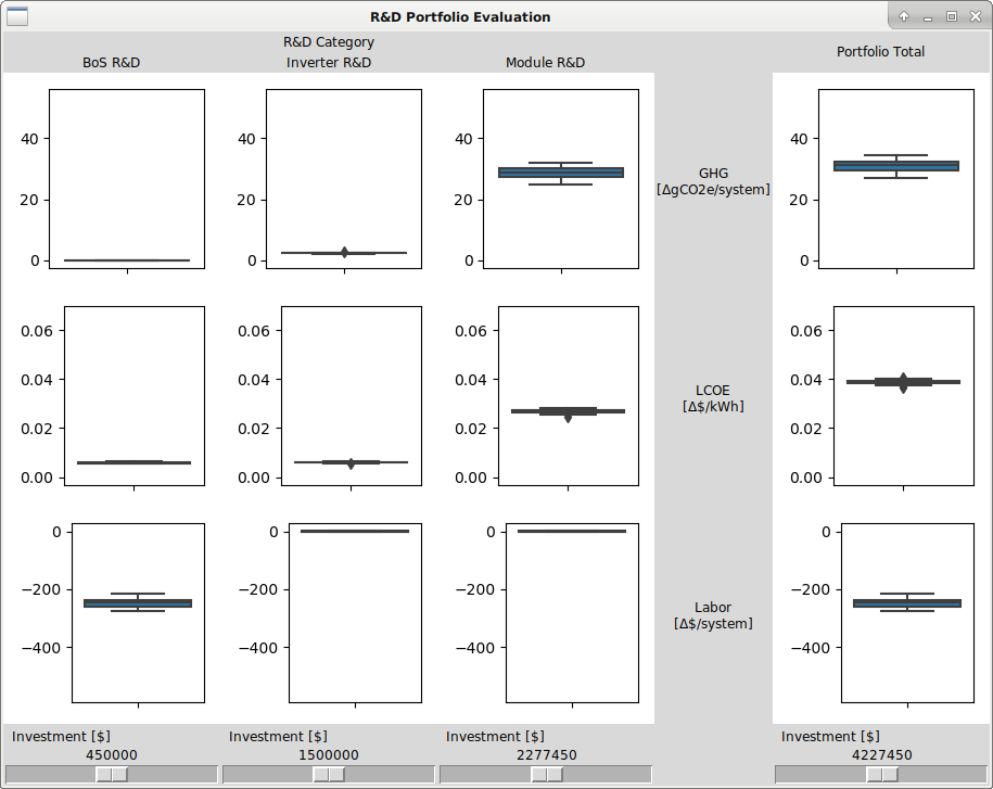
w = ty.DecisionWindow(evaluator)
w.mainloop()

A new window should open that looks like the image below. Moving the sliders will cause a recomputation of the boxplots.

Image("pv_residential_simple_gui.png")