LCSS Example

An example of using the LCSSMatcher to match a gps trace to the Open Street Maps road network

%%capture
!pip install mappymatch

from mappymatch import package_root

First, we load the trace from a file. The mappymatch package has a few sample traces included that we can use for demonstration.

Before we build the trace, though, let's take a look at the file to see how mappymatch expects the input data:

import pandas as pd

df = pd.read_csv(package_root() / "resources/traces/sample_trace_3.csv")
df.head()

	latitude	longitude
0	39.655210	-104.919169
1	39.655449	-104.919274
2	39.655690	-104.919381
3	39.655936	-104.919486
4	39.656182	-104.919593

Notice that we expect the input data to be in the EPSG:4326 coordinate reference system. If your input data is not in this format, you'll need to convert it prior to building a Trace object.

In order to idenfiy which coordinate is which in a trace, mappymatch uses the dataframe index as the coordinate index and so in this case, we just have a simple range based index for each coordinate. We could set a different index on the dataframe and mappymatch would use that to identify the coordinates.

Now, let's load the trace from the same file:

from mappymatch.constructs.trace import Trace

trace = Trace.from_csv(
    package_root() / "resources/traces/sample_trace_3.csv",
    lat_column="latitude",
    lon_column="longitude",
    xy=True,
)

Notice here that we pass three optional arguments to the from_csv function. By default, mappymatch expects the latitude and longitude columns to be named "latitude" and "longitude" but you can pass your own values if needed. Also by default, mappymatch converts the trace into the web mercator coordinate reference system (EPSG:3857) by setting xy=True. The LCSS matcher computes the cartesian distance between geometries and so a projected coordiante reference system is ideal. In a future version of mappymatch we hope to support any projected coordiante system but right now we only support EPSG:3857.

Okay, let's plot the trace to see what it looks like (mappymatch uses folium under the hood for plotting):

from mappymatch.utils.plot import plot_trace

plot_trace(trace, point_color="black", line_color="yellow")

Make this Notebook Trusted to load map: File -> Trust Notebook

Next, we need to get a road map to match our Trace to. One way to do this is to build a small geofence around the trace and then download a map that just fits around our trace:

from mappymatch.constructs.geofence import Geofence

geofence = Geofence.from_trace(trace, padding=2e3)

Notice that we pass an optional argument to the constructor. The padding defines how large around the trace we should build our geofence and is in the same units as the trace. In our case, the trace has been projected to the web mercator CRS and so our units would be in approximate meters, 1e3 meters or 1 kilomter

Now, let's plot both the trace and the geofence:

from mappymatch.utils.plot import plot_geofence

plot_trace(trace, point_color="black", m=plot_geofence(geofence))

Make this Notebook Trusted to load map: File -> Trust Notebook

At this point, we're ready to download a road network. Mappymatch has a couple of ways to represent a road network: The NxMap and the IGraphMap which use networkx and igraph, respectively, under the hood to represent the road graph structure. You might experiment with both to see if one is more performant or memory efficient in your use case.

In this example we'll use the NxMap:

from mappymatch.maps.nx.nx_map import NxMap, NetworkType

nx_map = NxMap.from_geofence(
    geofence,
    network_type=NetworkType.DRIVE,
)

{'osmid': 16983030, 'highway': 'residential', 'name': 'East Asbury Avenue', 'oneway': False, 'reversed': True, 'length': 79.54373679802445, 'speed_kph': 39.947450386398764, 'travel_time': 7.168353667206419, 'kilometers': 0.07954373679802446}
{'osmid': 16983030, 'highway': 'residential', 'name': 'East Asbury Avenue', 'oneway': False, 'reversed': False, 'length': 79.54373679802445, 'speed_kph': 39.947450386398764, 'travel_time': 7.168353667206419, 'kilometers': 0.07954373679802446}
{'osmid': 16986821, 'highway': 'residential', 'name': 'East Vassar Avenue', 'oneway': False, 'reversed': True, 'length': 83.64761710826589, 'speed_kph': 39.947450386398764, 'travel_time': 7.538188762411878, 'kilometers': 0.08364761710826589}
{'osmid': 16986821, 'highway': 'residential', 'name': 'East Vassar Avenue', 'oneway': False, 'reversed': False, 'length': 83.64761710826589, 'speed_kph': 39.947450386398764, 'travel_time': 7.538188762411878, 'kilometers': 0.08364761710826589}
{'osmid': 234196398, 'highway': 'secondary', 'lanes': '5', 'maxspeed': '30 mph', 'name': 'East Yale Avenue', 'oneway': False, 'reversed': True, 'length': 20.542709041809864, 'speed_kph': 48.2802, 'travel_time': 1.531761520261215, 'kilometers': 0.020542709041809864}
{'osmid': 37886699, 'highway': 'secondary', 'lanes': '6', 'maxspeed': '30 mph', 'name': 'East Yale Avenue', 'oneway': False, 'reversed': False, 'length': 14.354081263098669, 'speed_kph': 48.2802, 'travel_time': 1.0703081707854403, 'kilometers': 0.014354081263098669}
{'osmid': 16984718, 'highway': 'residential', 'name': 'South Kirkwood Court', 'oneway': False, 'reversed': True, 'length': 32.08319603301365, 'speed_kph': 39.947450386398764, 'travel_time': 2.8912860420792765, 'kilometers': 0.03208319603301365}
{'osmid': 33105941, 'highway': 'residential', 'name': 'East Kentucky Avenue', 'oneway': False, 'reversed': False, 'length': 41.12338570051541, 'speed_kph': 39.947450386398764, 'travel_time': 3.7059733998007873, 'kilometers': 0.041123385700515415}
{'osmid': 33105941, 'highway': 'residential', 'name': 'East Kentucky Avenue', 'oneway': False, 'reversed': True, 'length': 41.12338570051541, 'speed_kph': 39.947450386398764, 'travel_time': 3.7059733998007873, 'kilometers': 0.041123385700515415}
{'osmid': 1176411245, 'highway': 'residential', 'maxspeed': '25 mph', 'name': 'South Pennsylvania Street', 'oneway': False, 'reversed': False, 'length': 207.47072269064134, 'speed_kph': 40.2335, 'travel_time': 18.563997705551564, 'kilometers': 0.20747072269064135}
Warning: found 1667 of 10622 links with no geometry; creating link geometries from the node endpoints

The from_geofence constructor uses the osmnx package under the hood to download a road network.

Notice we pass the optional argument network_type which defaults to NetworkType.DRIVE but can be used to get a different network like NetworkType.BIKE or NetworkType.WALK

Now, we can plot the map to make sure we have the network that we want to match to:

from mappymatch.utils.plot import plot_map

plot_map(nx_map)

Make this Notebook Trusted to load map: File -> Trust Notebook

Now, we're ready to perform the actual map matching.

In this example we'll use the LCSSMatcher which implements the algorithm described in this paper:

Zhu, Lei, Jacob R. Holden, and Jeffrey D. Gonder. "Trajectory Segmentation Map-Matching Approach for Large-Scale, High-Resolution GPS Data." Transportation Research Record: Journal of the Transportation Research Board 2645 (2017): 67-75.

We won't go into detail here for how to tune the paramters but checkout the referenced paper for more details if you're interested. The default parameters have been set based on internal testing on high resolution driving GPS traces.

from mappymatch.matchers.lcss.lcss import LCSSMatcher

matcher = LCSSMatcher(nx_map)

match_result = matcher.match_trace(trace)

Now that we have the results, let's plot them:

from mappymatch.utils.plot import plot_matches

plot_matches(match_result.matches)

Make this Notebook Trusted to load map: File -> Trust Notebook

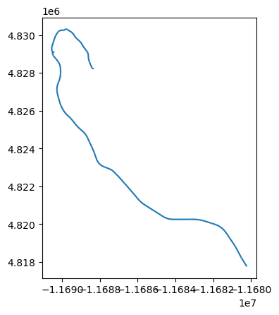
match_result.path_to_geodataframe().plot()

<Axes: >

The plot_matches function plots the roads that each point has been matched to and labels them with the road id.

In some cases, if the trace is much sparser (for example if it was collected a lower resolution), you might want see the estimated path, rather than the explict matched roads.

For example, let's reduce the trace frequency to every 30th point and re-match it:

reduced_trace = trace[0::30]

plot_trace(reduced_trace, point_color="black", line_color="yellow")

Make this Notebook Trusted to load map: File -> Trust Notebook

reduced_matches = matcher.match_trace(reduced_trace)

plot_matches(reduced_matches.matches)

Make this Notebook Trusted to load map: File -> Trust Notebook

The match result also has a path attribute with the estiamted path through the network:

from mappymatch.utils.plot import plot_path

plot_trace(
    reduced_trace, point_color="blue", m=plot_path(reduced_matches.path, crs=trace.crs)
)

Make this Notebook Trusted to load map: File -> Trust Notebook

Lastly, we might want to convert the results into a format more suitible for saving to file or merging with some other dataset. To do this, we can convert the result into a dataframe:

result_df = reduced_matches.matches_to_dataframe()
result_df.head()

	coordinate_id	distance_to_road	road_id	geom	origin_junction_id	destination_junction_id	road_key	kilometers	travel_time
0	0	18.704781	(432968976, 432968864, 0)	LINESTRING (-11679421.184827643 4815736.167510...	432968976	432968864	0	0.548364	26.861128
1	30	6.637295	(432968864, 176066679, 0)	LINESTRING (-11679700.006756231 4816391.715274...	432968864	176066679	0	0.713160	24.543028
2	60	5.474720	(176066679, 442605942, 0)	LINESTRING (-11680004.732730329 4817267.513675...	176066679	442605942	0	0.849679	29.241278
3	90	6.923850	(442615878, 442618319, 0)	LINESTRING (-11680833.539735131 4818830.551805...	442615878	442618319	0	0.424253	14.600453
4	120	7.800845	(442618319, 442617120, 0)	LINESTRING (-11681140.002293285 4819289.434003...	442618319	442617120	0	0.957481	34.269262

Here, for each coordinate, we have the distance to the matched road, and then attributes of the road itself like the geometry, the OSM node id and the road distance and travel time.

We can also get a dataframe for the path:

path_df = reduced_matches.path_to_dataframe()
path_df.head()

	road_id	geom	origin_junction_id	destination_junction_id	road_key	kilometers	travel_time
0	(432968976, 432968864, 0)	LINESTRING (-11679421.184827643 4815736.167510...	432968976	432968864	0	0.548364	26.861128
1	(432968864, 176066679, 0)	LINESTRING (-11679700.006756231 4816391.715274...	432968864	176066679	0	0.713160	24.543028
2	(176066679, 442605942, 0)	LINESTRING (-11680004.732730329 4817267.513675...	176066679	442605942	0	0.849679	29.241278
3	(442605942, 442615878, 0)	LINESTRING (-11680517.325589584 4818246.301911...	442605942	442615878	0	0.510779	17.578186
4	(442615878, 442618319, 0)	LINESTRING (-11680833.539735131 4818830.551805...	442615878	442618319	0	0.424253	14.600453

Another thing we can do is to only get a certain set of road types to match to. For example, let's say I only want to consider highways and primary roads for matching, I can do so by passing a custom filter when building the road network:

nx_map = NxMap.from_geofence(
    geofence,
    network_type=NetworkType.DRIVE,
    custom_filter='["highway"~"motorway|primary"]',
)

{'osmid': 427708173, 'highway': 'motorway_link', 'lanes': '2', 'oneway': True, 'reversed': False, 'length': 20.414537964823523, 'speed_kph': 74.37609513888889, 'travel_time': 0.9881177081981263, 'kilometers': 0.020414537964823523}
{'osmid': 344391013, 'highway': 'motorway_link', 'lanes': '1', 'oneway': True, 'reversed': False, 'length': 22.563432845186533, 'speed_kph': 74.37609513888889, 'travel_time': 1.0921299120501933, 'kilometers': 0.022563432845186533}
{'osmid': 177242486, 'highway': 'motorway_link', 'lanes': '3', 'oneway': True, 'reversed': False, 'length': 20.12349405707779, 'speed_kph': 74.37609513888889, 'travel_time': 0.974030412193569, 'kilometers': 0.02012349405707779}
{'osmid': 186241519, 'highway': 'primary', 'lanes': '4', 'maxspeed': '35 mph', 'name': 'South Colorado Boulevard', 'oneway': True, 'ref': 'CO 2', 'reversed': False, 'length': 12.226081069694452, 'speed_kph': 56.3269, 'travel_time': 0.7814009265714965, 'kilometers': 0.012226081069694451}
{'osmid': 132231509, 'highway': 'motorway', 'lanes': '4', 'maxspeed': '55 mph', 'name': 'West 6th Avenue Freeway', 'oneway': True, 'reversed': False, 'length': 58.72923421018891, 'speed_kph': 88.5137, 'travel_time': 2.388616035220312, 'kilometers': 0.05872923421018891}
{'osmid': 520031957, 'highway': 'motorway_link', 'lanes': '1', 'oneway': True, 'reversed': False, 'length': 197.08499535304279, 'speed_kph': 74.37609513888889, 'travel_time': 9.539435781698844, 'kilometers': 0.1970849953530428}
{'osmid': 16982076, 'highway': 'primary_link', 'lanes': '1', 'oneway': True, 'ref': 'US 287', 'reversed': False, 'length': 119.30913844814366, 'speed_kph': 72.77331257167408, 'travel_time': 5.902066062889359, 'kilometers': 0.11930913844814366}
{'osmid': 646049993, 'highway': 'primary_link', 'lanes': '1', 'oneway': False, 'reversed': False, 'length': 14.763038968321924, 'speed_kph': 72.77331257167408, 'travel_time': 0.7303081089460475, 'kilometers': 0.014763038968321924}
{'osmid': 645821551, 'highway': 'primary_link', 'lanes': '1', 'oneway': False, 'reversed': False, 'length': 12.546375003231507, 'speed_kph': 72.77331257167408, 'travel_time': 0.6206526598215344, 'kilometers': 0.012546375003231507}
{'osmid': 646049993, 'highway': 'primary_link', 'lanes': '1', 'oneway': False, 'reversed': True, 'length': 14.763038968321924, 'speed_kph': 72.77331257167408, 'travel_time': 0.7303081089460475, 'kilometers': 0.014763038968321924}
Warning: found 46 of 388 links with no geometry; creating link geometries from the node endpoints

plot_map(nx_map)

Make this Notebook Trusted to load map: File -> Trust Notebook

Above you can see that now we have a much reduced graph to match to, let's see what happens

matcher = LCSSMatcher(nx_map)

match_result = matcher.match_trace(trace)

plot_matches(match_result.matches)

Make this Notebook Trusted to load map: File -> Trust Notebook

plot_path(match_result.path, crs=trace.crs)

Make this Notebook Trusted to load map: File -> Trust Notebook

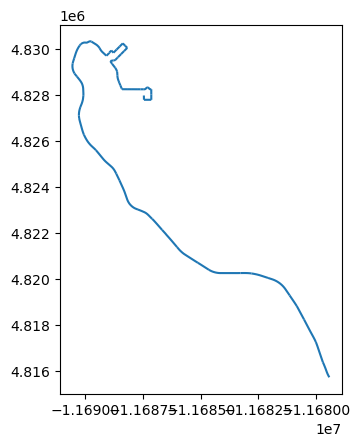
path_gdf = match_result.path_to_geodataframe()

path_gdf.plot()

<Axes: >