
[ ]:
# This information helps with debugging and getting support :)
import sys, platform
import pandas as pd
import bifacial_radiance as br
print("Working on a ", platform.system(), platform.release())
print("Python version ", sys.version)
print("Pandas version ", pd.__version__)
print("bifacial_radiance version ", br.__version__)
11 - AgriPV Systems#
This journal shows how to model an AgriPV site, calculating the irradiance not only on the modules but also the irradiance received by the ground to evaluate available solar ersource for plants.
We assume that bifacia_radiacne is already installed in your computer. This works for bifacial_radiance v.3 release.
These journal outlines 4 useful uses of bifacial_radiance and some tricks:
Creating the modules in the AgriPV site
Adding extra geometry for the pillars/posts supporting the AgriPV site
Hacking the sensors to sample the ground irradiance and create irradiance map
Adding object to simulate variations in ground albedo from different crops between rows.
Steps:#
Generate the geometry
Analyse the Ground Irradiance
Analyse and MAP the Ground Irradiance
Adding different Albedo Section
Preview of what we will create:#
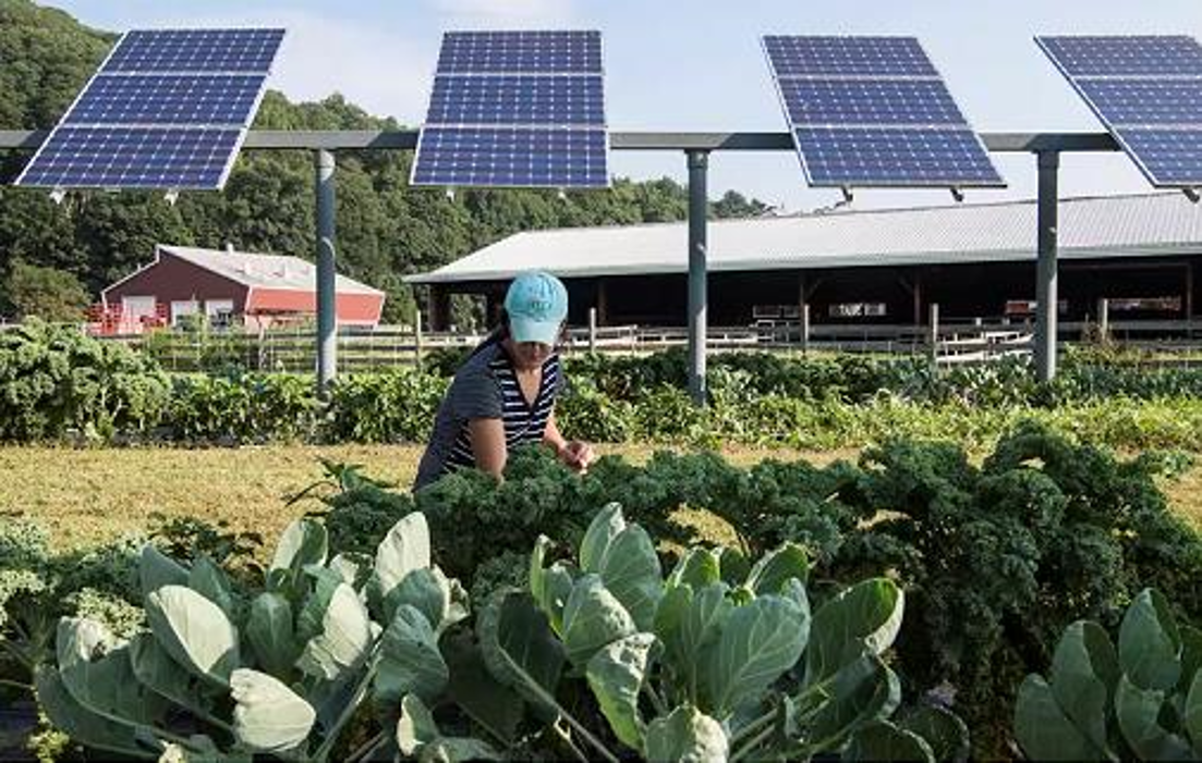
 And this is how it will look like:
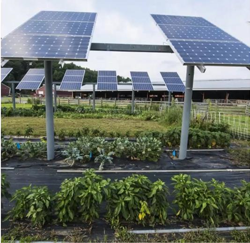
1. Generate the geometry#
This section goes from setting up variables to making the OCT axis. We are also adding some custom elements for the torquetubes and posts.
We’ve done this before a couple times, no new stuff here.
The magic is that, for doing the carport we see in the figure, we are going to do a 4-up configuration of modules (numpanels), and we are going to repeat that 3-UP 6 times (nMods)
[1]:
import os
from pathlib import Path

testfolder = str(Path().resolve().parent.parent / 'bifacial_radiance' / 'TEMP' /  'Tutorial_11')

if not os.path.exists(testfolder):
    os.makedirs(testfolder)

print ("Your simulation will be stored in %s" % testfolder)
Your simulation will be stored in C:\Users\mprillim\sam_dev\bifacial_radiance\bifacial_radiance\TEMP\Tutorial_11
[2]:
from bifacial_radiance import *
import numpy as np
import pandas as pd
[3]:
simulationname = 'tutorial_11'
#Location:
lat = 40.0583 # NJ
lon = -74.4057 # NJ
# MakeModule Parameters
moduletype='test-module'
numpanels = 3 # AgriPV site has 3 modules along the y direction (N-S since we are facing it to the south) .
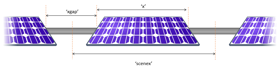
x = 0.95
y = 1.95
xgap = 2.0# Leaving 15 centimeters between modules on x direction
ygap = 0.10 # Leaving 10 centimeters between modules on y direction
zgap = 0 # no gap to torquetube.
sensorsy = 6*numpanels # this will give 6 sensors per module, 1 per cell
# Other default values:
# TorqueTube Parameters
axisofrotationTorqueTube=False # this is False by default if there is no torquetbue parameters
torqueTube = False
cellLevelModule = True
numcellsx = 12
numcellsy = 6
xcell = 0.156
ycell = 0.156
xcellgap = 0.02
ycellgap = 0.02
cellLevelModuleParams = {'numcellsx': numcellsx, 'numcellsy':numcellsy,
'xcell': xcell, 'ycell': ycell, 'xcellgap': xcellgap, 'ycellgap': ycellgap}
# SceneDict Parameters
pitch = 15 # m
albedo = 0.2 #'grass' # ground albedo
hub_height = 4.3 # m
nMods = 6 # six modules per row.
nRows = 3 # 3 row
azimuth_ang=180 # Facing south
tilt =35 # tilt.
# Now let's run the example
demo = RadianceObj(simulationname,path = testfolder)
demo.setGround(albedo)
epwfile = demo.getEPW(lat, lon) # NJ lat/lon 40.0583° N, 74.4057
metdata = demo.readWeatherFile(epwfile, coerce_year=2001)
timestamp = metdata.datetime.index(pd.to_datetime('2001-06-17 13:0:0 -5')) # Make this timezone aware, use -5 for EST.
demo.gendaylit(timestamp)
# Making module with all the variables
module=demo.makeModule(name=moduletype,x=x,y=y,numpanels=numpanels,
xgap=xgap, ygap=ygap, cellModule=cellLevelModuleParams)
# create a scene with all the variables
sceneDict = {'tilt':tilt,'pitch': 15,'hub_height':hub_height,'azimuth':azimuth_ang, 'nMods': nMods, 'nRows': nRows}
scene = demo.makeScene(module=moduletype, sceneDict=sceneDict)
octfile = demo.makeOct(demo.getfilelist())
path = C:\Users\mprillim\sam_dev\bifacial_radiance\bifacial_radiance\TEMP\Tutorial_11
Loading albedo, 1 value(s), 0.200 avg
1 nonzero albedo values.
Getting weather file: USA_NJ_McGuire.AFB.724096_TMY3.epw
 ... OK!
8760 line in WeatherFile. Assuming this is a standard hourly WeatherFile for the year for purposes of saving Gencumulativesky temporary weather files in EPW folder.
Coercing year to 2001
Saving file EPWs\metdata_temp.csv, # points: 8760
Calculating Sun position for Metdata that is right-labeled  with a delta of -30 mins. i.e. 12 is 11:30 sunpos

Module Name: test-module
Module was shifted by 0.078 in X to avoid sensors on air
This is a Cell-Level detailed module with Packaging Factor of 0.81 %
Module test-module updated in module.json
Pre-existing .rad file objects\test-module.rad will be overwritten

Created tutorial_11.oct
If desired, you can view the Oct file at this point:
rvu -vf views:nbsphinx-math:`front`.vp -e .01 tutorial_11.oct
[4]:
## Comment the ! line below to run rvu from the Jupyter notebook instead of your terminal.
## Simulation will stop until you close the rvu window

#!rvu -vf views\front.vp -e .01 tutorial_11.oct
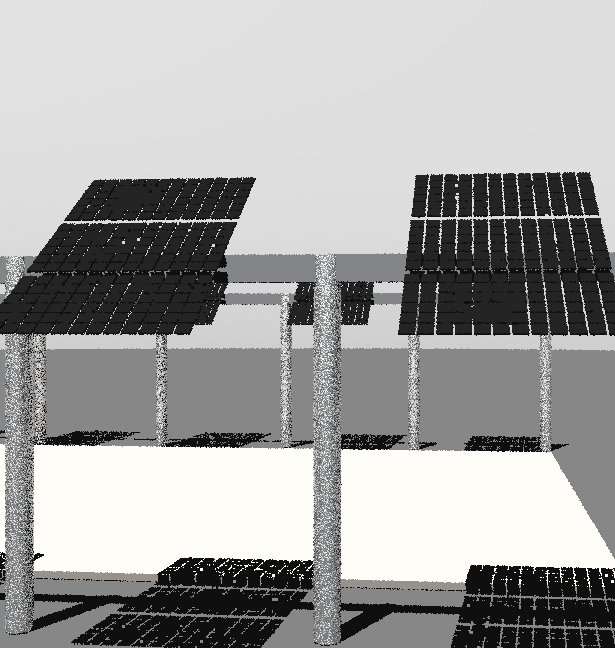
And adjust the view parameters, you should see this image.
Adding the structure#
We will add on the torquetube and pillars.
Positions of the piles could be done more programatically, but they are kinda estimated at the moment.
[5]:
torquetubelength = module.scenex*(nMods)

name='Post1'
text='! genbox Metal_Aluminum_Anodized torquetube_row1 {} 0.2 0.3 | xform -t {} -0.1 -0.3 | xform -t 0 0 4.2'.format(
                                                    torquetubelength, (-torquetubelength+module.sceney)/2.0)
customObject = demo.makeCustomObject(name,text)
demo.appendtoScene(radfile=scene.radfiles, customObject=customObject, text="!xform -rz 0")

name='Post2'
text='! genbox Metal_Aluminum_Anodized torquetube_row2 {} 0.2 0.3 | xform -t {} -0.1 -0.3 | xform -t 0 15 4.2'.format(
                                            torquetubelength, (-torquetubelength+module.sceney)/2.0)
customObject = demo.makeCustomObject(name,text)
demo.appendtoScene(radfile=scene.radfiles, customObject=customObject, text="!xform -rz 0")

name='Post3'
text='! genbox Metal_Aluminum_Anodized torquetube_row2 {} 0.2 0.3 | xform -t {} -0.1 -0.3 | xform -t 0 -15 4.2'.format(
                                              torquetubelength, (-torquetubelength+module.sceney)/2.0)
customObject = demo.makeCustomObject(name,text)
demo.appendtoScene(radfile=scene.radfiles, customObject=customObject, text="!xform -rz 0")
Custom Object Name objects\Post1.rad

Custom Object Name objects\Post2.rad

Custom Object Name objects\Post3.rad
[6]:
name='Pile'
pile1x = (torquetubelength+module.sceney)/2.0
pilesep = pile1x*2.0/7.0

text= '! genrev Metal_Grey tube1row1 t*4.2 0.15 32 | xform -t {} 0 0'.format(pile1x)
text += '\r\n! genrev Metal_Grey tube1row2 t*4.2 0.15 32 | xform -t {} 15 0'.format(pile1x)
text += '\r\n! genrev Metal_Grey tube1row3 t*4.2 0.15 32 | xform -t {} -15 0'.format(pile1x)

for i in range (1, 7):
    text += '\r\n! genrev Metal_Grey tube{}row1 t*4.2 0.15 32 | xform -t {} 0 0'.format(i+1, pile1x-pilesep*i)
    text += '\r\n! genrev Metal_Grey tube{}row2 t*4.2 0.15 32 | xform -t {} 15 0'.format(i+1, pile1x-pilesep*i)
    text += '\r\n! genrev Metal_Grey tube{}row3 t*4.2 0.15 32 | xform -t {} -15 0'.format(i+1, pile1x-pilesep*i)

customObject = demo.makeCustomObject(name,text)
demo.appendtoScene(radfile=scene.radfiles, customObject=customObject, text="!xform -rz 0")

octfile = demo.makeOct()  # makeOct combines all of the ground, sky and object files we just added into a .oct file.
Custom Object Name objects\Pile.rad
Created tutorial_11.oct
View the geometry with the posts on :#
rvu -vf views:nbsphinx-math:`front`.vp -e .01 -pe 0.4 -vp 12 -10 3.5 -vd -0.0995 0.9950 0.0 tutorial_11.oct
[7]:
## Comment the ! line below to run rvu from the Jupyter notebook instead of your terminal.
## Simulation will stop until you close the rvu window

#!rvu -vf views\front.vp -e .01 tutorial_11.oct

2. Analyse the Ground Irradiance#
Now let’s do some analysis along the ground, starting from the edge of the modules. We wil select to start in the center of the array.
We are also increasign the number of points sampled accross the collector width, with the variable sensorsy passed to moduleanalysis. We are also increasing the step between sampling points, to be able to sample in between the rows.
[8]:
analysis = AnalysisObj(octfile, demo.name)
sensorsy = 20
frontscan, backscan = analysis.moduleAnalysis(scene, sensorsy=sensorsy)
[9]:
groundscan = frontscan
[10]:
groundscan['zstart'] = 0.05  # setting it 5 cm from the ground.
groundscan['zinc'] = 0   # no tilt necessary.
groundscan['yinc'] = pitch/(sensorsy-1)   # increasing spacing so it covers all distance between rows
groundscan
[10]:
{'xstart': 1.5159739062663865e-16,
 'ystart': -1.237886635821746,
 'zstart': 0.05,
 'xinc': -1.5802346387185998e-17,
 'yinc': 0.7894736842105263,
 'zinc': 0,
 'sx_xinc': 0.0,
 'sx_yinc': 0.0,
 'sx_zinc': 0.0,
 'Nx': 1,
 'Ny': 20,
 'Nz': 1,
 'orient': '-0.000 0.574 -0.819'}
[11]:
analysis.analysis(octfile, simulationname+"_groundscan", groundscan, backscan) # compare the back vs front irradiance
Linescan in process: tutorial_11_groundscan_Front
Linescan in process: tutorial_11_groundscan_Back
Saved: results\irr_tutorial_11_groundscan.csv
[11]:
({'Wm2': [707.7193666666666,
   679.3139666666666,
   320.71520000000004,
   321.5017,
   326.947,
   355.2678,
   703.1252000000001,
   717.6289666666667,
   730.9323333333333,
   738.5453666666667,
   744.1402333333334,
   748.625,
   750.1326666666668,
   753.2622333333334,
   754.2802333333333,
   753.4847333333332,
   749.6281333333333,
   744.2707333333334,
   730.8705333333334,
   709.3668333333334],
  'x': [1.515974e-16,
   1.35795e-16,
   1.199927e-16,
   1.041904e-16,
   8.838801e-17,
   7.258566e-17,
   5.678331e-17,
   4.098097e-17,
   2.517862e-17,
   9.376273e-18,
   -6.426073e-18,
   -2.222842e-17,
   -3.803077e-17,
   -5.383311e-17,
   -6.963546e-17,
   -8.543781e-17,
   -1.012402e-16,
   -1.170425e-16,
   -1.328448e-16,
   -1.486472e-16],
  'y': [-1.237887,
   -0.448413,
   0.3410607,
   1.130534,
   1.920008,
   2.709482,
   3.498955,
   4.288429,
   5.077903,
   5.867377,
   6.65685,
   7.446324,
   8.235798,
   9.025271,
   9.814745,
   10.60422,
   11.39369,
   12.18317,
   12.97264,
   13.76211],
  'z': [0.05,
   0.05,
   0.05,
   0.05,
   0.05,
   0.05,
   0.05,
   0.05,
   0.05,
   0.05,
   0.05,
   0.05,
   0.05,
   0.05,
   0.05,
   0.05,
   0.05,
   0.05,
   0.05,
   0.05],
  'r': [707.5753,
   679.1962,
   320.6044,
   321.3819,
   326.8311,
   355.1729,
   703.0397,
   717.5341,
   730.8545,
   738.4874,
   744.0706,
   748.5612,
   750.0686,
   753.1605,
   754.1783,
   753.3657,
   749.512,
   744.1373,
   730.7393,
   709.2124],
  'g': [707.7124,
   679.3104,
   320.7099,
   321.4949,
   326.9389,
   355.2608,
   703.1177,
   717.6204,
   730.9257,
   738.5405,
   744.1342,
   748.6193,
   750.127,
   753.2527,
   754.2706,
   753.4746,
   749.619,
   744.2607,
   730.8623,
   709.3582],
  'b': [707.8704,
   679.4353,
   320.8313,
   321.6283,
   327.071,
   355.3697,
   703.2182,
   717.7324,
   731.0168,
   738.6082,
   744.2159,
   748.6945,
   750.2024,
   753.3735,
   754.3918,
   753.6139,
   749.7534,
   744.4142,
   731.01,
   709.5299],
  'mattype': ['groundplane',
   'groundplane',
   'groundplane',
   'groundplane',
   'groundplane',
   'groundplane',
   'groundplane',
   'groundplane',
   'groundplane',
   'groundplane',
   'groundplane',
   'groundplane',
   'groundplane',
   'groundplane',
   'groundplane',
   'groundplane',
   'groundplane',
   'groundplane',
   'groundplane',
   'groundplane'],
  'title': 'tutorial_11_groundscan_Front'},
 {'Wm2': [258.8127,
   131.0589,
   130.75906666666668,
   130.4594,
   125.61353333333334,
   124.4103,
   258.8127,
   100.8693,
   87.56585,
   81.7781,
   135.29413333333335,
   127.25869999999999,
   129.3859666666667,
   258.8127,
   132.0198,
   133.18776666666668,
   134.2764,
   135.00026666666668,
   135.94163333333333,
   258.8127],
  'x': [1.50052e-16,
   1.342497e-16,
   1.184474e-16,
   1.02645e-16,
   8.684266e-17,
   7.104032e-17,
   5.523797e-17,
   3.943562e-17,
   2.363328e-17,
   7.83093e-18,
   -7.971416e-18,
   -2.377376e-17,
   -3.957611e-17,
   -5.537846e-17,
   -7.11808e-17,
   -8.698315e-17,
   -1.027855e-16,
   -1.185878e-16,
   -1.343902e-16,
   -1.501925e-16],
  'y': [-1.225268,
   -1.096232,
   -0.9671961,
   -0.8381601,
   -0.7091242,
   -0.5800882,
   -0.4510523,
   -0.3220163,
   -0.1929803,
   -0.0639444,
   0.06509155,
   0.1941275,
   0.3231635,
   0.4521994,
   0.5812354,
   0.7102713,
   0.8393073,
   0.9683432,
   1.097379,
   1.226415],
  'z': [3.440837,
   3.531189,
   3.621541,
   3.711893,
   3.802245,
   3.892597,
   3.982949,
   4.073301,
   4.163653,
   4.254005,
   4.344357,
   4.434709,
   4.525061,
   4.615413,
   4.705765,
   4.796117,
   4.886468,
   4.97682,
   5.067172,
   5.157524],
  'r': [258.8127,
   130.8674,
   130.568,
   130.2688,
   125.3934,
   124.1923,
   258.8127,
   100.1214,
   86.4007,
   80.33697,
   134.2312,
   126.7886,
   128.908,
   258.8127,
   131.8432,
   133.0096,
   134.1148,
   134.8378,
   135.8387,
   258.8127],
  'g': [258.8127,
   131.0518,
   130.752,
   130.4523,
   125.5993,
   124.3962,
   258.8127,
   100.7859,
   87.42799,
   81.59953,
   135.1632,
   127.206,
   129.3324,
   258.8127,
   132.0045,
   133.1724,
   134.2626,
   134.9864,
   135.9336,
   258.8127],
  'b': [258.8127,
   131.2575,
   130.9572,
   130.6571,
   125.8479,
   124.6424,
   258.8127,
   101.7006,
   88.86886,
   83.3978,
   136.488,
   127.7815,
   129.9175,
   258.8127,
   132.2117,
   133.3813,
   134.4518,
   135.1766,
   136.0526,
   258.8127],
  'mattype': ['sky',
   'a2.1.a5.1.0.cellPVmodule.2310',
   'a2.1.a5.2.0.cellPVmodule.2310',
   'a2.1.a5.3.0.cellPVmodule.2310',
   'a2.1.a5.4.0.cellPVmodule.2310',
   'a2.1.a5.5.0.cellPVmodule.2310',
   'sky',
   'a2.1.a5.0.1.cellPVmodule.2310',
   'a2.1.a5.1.1.cellPVmodule.2310',
   'a2.1.a5.2.1.cellPVmodule.2310',
   'a2.1.a5.3.1.cellPVmodule.2310',
   'a2.1.a5.4.1.cellPVmodule.2310',
   'a2.1.a5.5.1.cellPVmodule.2310',
   'sky',
   'a2.1.a5.0.2.cellPVmodule.2310',
   'a2.1.a5.1.2.cellPVmodule.2310',
   'a2.1.a5.2.2.cellPVmodule.2310',
   'a2.1.a5.3.2.cellPVmodule.2310',
   'a2.1.a5.4.2.cellPVmodule.2310',
   'sky'],
  'title': 'tutorial_11_groundscan_Back'})
This is the result for only one ‘chord’ accross the ground. Let’s now do a X-Y scan of the ground.
3. Analyse and MAP the Ground Irradiance#
We will use the same technique to find the irradiance on the ground used above, but will move it along the X-axis to map from the start of one module to the next.
We will sample around the module that is placed at the center of the field.
[12]:
import seaborn as sns
[13]:
sensorsx = 20
startgroundsample=-module.scenex
spacingbetweensamples = module.scenex/(sensorsx-1)

for i in range (0, sensorsx): # Will map 20 points
    frontscan, backscan = analysis.moduleAnalysis(scene, sensorsy=sensorsy)
    groundscan = frontscan
    groundscan['zstart'] = 0.05  # setting it 5 cm from the ground.
    groundscan['zinc'] = 0   # no tilt necessary.
    groundscan['yinc'] = pitch/(sensorsy-1)   # increasing spacing so it covers all distance between rows
    groundscan['xstart'] = startgroundsample + i*spacingbetweensamples   # increasing spacing so it covers all distance between rows
    analysis.analysis(octfile, simulationname+"_groundscan_"+str(i), groundscan, backscan)  # compare the back vs front irradiance
Linescan in process: tutorial_11_groundscan_0_Front
Linescan in process: tutorial_11_groundscan_0_Back
Saved: results\irr_tutorial_11_groundscan_0.csv
Linescan in process: tutorial_11_groundscan_1_Front
Linescan in process: tutorial_11_groundscan_1_Back
Saved: results\irr_tutorial_11_groundscan_1.csv
Linescan in process: tutorial_11_groundscan_2_Front
Linescan in process: tutorial_11_groundscan_2_Back
Saved: results\irr_tutorial_11_groundscan_2.csv
Linescan in process: tutorial_11_groundscan_3_Front
Linescan in process: tutorial_11_groundscan_3_Back
Saved: results\irr_tutorial_11_groundscan_3.csv
Linescan in process: tutorial_11_groundscan_4_Front
Linescan in process: tutorial_11_groundscan_4_Back
Saved: results\irr_tutorial_11_groundscan_4.csv
Linescan in process: tutorial_11_groundscan_5_Front
Linescan in process: tutorial_11_groundscan_5_Back
Saved: results\irr_tutorial_11_groundscan_5.csv
Linescan in process: tutorial_11_groundscan_6_Front
Linescan in process: tutorial_11_groundscan_6_Back
Saved: results\irr_tutorial_11_groundscan_6.csv
Linescan in process: tutorial_11_groundscan_7_Front
Linescan in process: tutorial_11_groundscan_7_Back
Saved: results\irr_tutorial_11_groundscan_7.csv
Linescan in process: tutorial_11_groundscan_8_Front
Linescan in process: tutorial_11_groundscan_8_Back
Saved: results\irr_tutorial_11_groundscan_8.csv
Linescan in process: tutorial_11_groundscan_9_Front
Linescan in process: tutorial_11_groundscan_9_Back
Saved: results\irr_tutorial_11_groundscan_9.csv
Linescan in process: tutorial_11_groundscan_10_Front
Linescan in process: tutorial_11_groundscan_10_Back
Saved: results\irr_tutorial_11_groundscan_10.csv
Linescan in process: tutorial_11_groundscan_11_Front
Linescan in process: tutorial_11_groundscan_11_Back
Saved: results\irr_tutorial_11_groundscan_11.csv
Linescan in process: tutorial_11_groundscan_12_Front
Linescan in process: tutorial_11_groundscan_12_Back
Saved: results\irr_tutorial_11_groundscan_12.csv
Linescan in process: tutorial_11_groundscan_13_Front
Linescan in process: tutorial_11_groundscan_13_Back
Saved: results\irr_tutorial_11_groundscan_13.csv
Linescan in process: tutorial_11_groundscan_14_Front
Linescan in process: tutorial_11_groundscan_14_Back
Saved: results\irr_tutorial_11_groundscan_14.csv
Linescan in process: tutorial_11_groundscan_15_Front
Linescan in process: tutorial_11_groundscan_15_Back
Saved: results\irr_tutorial_11_groundscan_15.csv
Linescan in process: tutorial_11_groundscan_16_Front
Linescan in process: tutorial_11_groundscan_16_Back
Saved: results\irr_tutorial_11_groundscan_16.csv
Linescan in process: tutorial_11_groundscan_17_Front
Linescan in process: tutorial_11_groundscan_17_Back
Saved: results\irr_tutorial_11_groundscan_17.csv
Linescan in process: tutorial_11_groundscan_18_Front
Linescan in process: tutorial_11_groundscan_18_Back
Saved: results\irr_tutorial_11_groundscan_18.csv
Linescan in process: tutorial_11_groundscan_19_Front
Linescan in process: tutorial_11_groundscan_19_Back
Saved: results\irr_tutorial_11_groundscan_19.csv
Read all the files generated into one dataframe
[14]:
filestarter = "irr_tutorial_11_groundscan_"

filelist = sorted(os.listdir(os.path.join(testfolder, 'results')))
prefixed = [filename for filename in filelist if filename.startswith(filestarter)]
arrayWm2Front = []
arrayWm2Back = []
arrayMatFront = []
arrayMatBack = []
filenamed = []
faillist = []

print('{} files in the directory'.format(filelist.__len__()))
print('{} groundscan files in the directory'.format(prefixed.__len__()))
i = 0  # counter to track # files loaded.

for i in range (0, len(prefixed)):
    ind = prefixed[i].split('_')

    try:
        resultsDF = load.read1Result(os.path.join(testfolder, 'results', prefixed[i]))
        arrayWm2Front.append(list(resultsDF['Wm2Front']))
        arrayWm2Back.append(list(resultsDF['Wm2Back']))
        arrayMatFront.append(list(resultsDF['mattype']))
        arrayMatBack.append(list(resultsDF['rearMat']))
        filenamed.append(prefixed[i])
    except:
        print(" FAILED ", i, prefixed[i])
        faillist.append(prefixed[i])

resultsdf = pd.DataFrame(list(zip(arrayWm2Front, arrayWm2Back,
                                  arrayMatFront, arrayMatBack)),
                         columns = ['br_Wm2Front', 'br_Wm2Back',
                                    'br_MatFront', 'br_MatBack'])
resultsdf['filename'] = filenamed
21 files in the directory
20 groundscan files in the directory
Creating a new dataframe where each element in the front irradiance list is a column. Also transpose and reverse so it looks like a top-down view of the ground.
[15]:
df3 = pd.DataFrame(resultsdf['br_Wm2Front'].to_list())
reversed_df = df3.T.iloc[::-1]
[16]:
sns.set(rc={'figure.figsize':(11.7,8.27)})
print(sns)
<module 'seaborn' from 'C:\\Users\\mprillim\\AppData\\Local\\anaconda3\\Lib\\site-packages\\seaborn\\__init__.py'>
[17]:
# Plot
print(reversed_df)
ax = sns.heatmap(reversed_df)
ax.set_yticks([])
ax.set_xticks([])
ax.set_ylabel('')
ax.set_xlabel('')
print('')
            0           1           2           3           4           5   \
19  706.103133  708.401400  721.409200  717.619833  715.598133  714.769967
18  729.545700  730.459500  736.484300  733.422067  733.810267  732.349067
17  744.611167  744.542333  744.579000  744.724633  750.426100  744.390300
16  750.814333  751.606700  749.812433  750.632400  751.096500  750.848633
15  753.168167  753.276833  753.276567  755.596267  752.409900  752.694000
14  755.519533  752.961300  752.966167  755.388967  753.513033  752.432300
13  754.755633  752.870133  752.360067  752.922700  752.463167  753.046767
12  750.480900  752.070000  750.826967  751.828333  751.950300  752.030000
11  748.509767  747.130000  749.399867  746.466000  748.227600  746.539433
10  745.415200  744.417000  743.864667  744.758867  744.103900  742.821967
9   738.088100  739.890267  741.674200  738.149167  737.464833  736.426367
8   731.910667  730.627967  729.591467  731.874200  731.301133  730.675900
7   720.658000  718.901000  720.356467  722.543900  721.599267  720.658700
6   705.715100  705.710900  705.746200  707.904900  707.941067  707.607633
5   355.021367  680.047933  687.220900  689.482767  688.437867  690.134767
4   338.137467  328.818467  669.616733  665.818167  669.199033  670.765433
3   320.249833  319.284800  320.558033  321.297400  320.372400  322.348033
2   327.381400  651.769900  275.794300  291.608000  650.141667  662.958800
1   675.499700  677.584933  705.427933  697.571600  690.976100  691.939233
0   709.134933  708.707133  715.170800  716.620033  715.826767  714.051933

            6           7           8           9           10          11  \
19  717.691533  711.522867  712.757500  710.257500  709.220933  709.313067
18  733.783333  735.913067  732.007233  733.509267  730.354000  727.958400
17  745.029333  743.979700  744.263733  743.381600  743.023400  744.490167
16  749.903167  751.742567  749.769567  751.066300  753.117233  751.002000
15  751.250233  752.366833  753.492867  753.876900  753.367467  751.385933
14  753.530700  754.778467  752.997567  753.582500  753.520900  754.236267
13  753.227333  753.807267  751.415867  752.906700  751.486333  753.493467
12  750.532067  750.670900  749.872667  750.832367  750.489133  750.151933
11  748.346967  748.892033  748.041633  749.023133  746.868867  749.238767
10  745.314000  743.720400  746.012533  743.005167  743.646567  744.196700
9   738.304500  739.222567  738.664833  738.182167  738.772300  736.990800
8   729.956467  731.690267  729.075000  732.476567  732.160167  728.579133
7   720.596533  717.014033  720.265167  721.179033  722.140600  718.498733
6   702.689367  704.966000  706.626000  704.748233  704.622767  701.180133
5   689.890667  687.784400  686.179433  681.387233  351.740667  350.329433
4   666.880300  669.387933  667.090400  664.898567  330.810567  328.805800
3   327.578400  324.940033  325.044300  326.605767  320.433933  316.942600
2   668.190433  666.299400  664.494500  330.880267  327.974767  327.230867
1   694.239867  687.681200  681.103600  680.670400  680.848533  675.766867
0   714.675833  711.183500  714.889300  708.400500  707.713700  706.633333

            12          13          14          15          16          17  \
19  706.175833  707.180167  707.157300  712.048733  711.981600  712.040900
18  730.764033  731.337400  730.642267  731.579567  732.021133  734.080200
17  744.146933  744.611200  744.521800  750.407100  744.508967  744.732367
16  751.809200  752.194033  751.928133  751.819000  752.302333  750.826333
15  755.611933  752.418633  753.354900  753.825367  754.609733  753.545500
14  755.459067  753.681333  752.879167  753.613000  754.177467  754.335200
13  752.477633  752.804200  752.309033  752.380667  752.349700  753.632500
12  751.937000  751.482567  751.690500  751.212533  750.968867  751.490867
11  745.877267  749.956467  746.414533  748.219567  747.418833  750.582933
10  743.980700  744.447867  744.451467  743.770867  744.250100  743.863700
9   738.769033  740.103767  739.964800  740.716233  740.526967  739.124967
8   731.160033  732.168800  732.826267  732.408633  729.162133  728.532900
7   720.710100  723.232600  719.786533  722.325033  721.168400  720.971133
6   701.214467  701.417100  705.849133  704.621900  703.753500  707.717633
5   352.463567  354.728900  349.988367  351.652033  352.812367  356.005000
4   326.716367  332.401600  657.308800  327.399467  332.307633  332.213533
3   315.542133  321.294167  316.153100  317.716767  319.481167  319.000733
2   322.115700  326.696033  325.644433  328.398267  334.000367  333.711533
1   678.285333  675.390400  680.057467  683.956267  684.276000  692.499100
0   707.710367  708.147867  708.910233  712.326833  712.278500  711.902933

            18          19
19  715.376667  717.643300
18  732.649500  733.783533
17  744.968867  745.995367
16  752.177467  749.564300
15  752.481233  754.267833
14  753.339100  753.756800
13  752.515900  752.555833
12  750.258367  751.863267
11  748.909267  747.531667
10  743.856633  743.706133
9   740.541067  740.049867
8   730.285833  731.056367
7   720.315467  720.296133
6   704.827100  705.745667
5   358.585133  685.921833
4   335.268367  665.815167
3   318.638567  324.686667
2   648.111033  627.050300
1   697.486433  704.735667
0   715.283367  718.631267

4. Adding different Albedo Sections#
Add a surface (just like we added the pillars) with a specific reflectivity to represent different albedo sections. In the image, we can see that the albedo between the crops is different than the crop albedo. Let’s assume that the abledo between the crops is higher than the crop’s albedo which wa previuosly set a 0.2.
[18]:
name='Center_Grass'
carpositionx=-2
carpositiony=-1
text='! genbox white_EPDM CenterPatch 28 12 0.1 | xform -t -14 2 0'.format(carpositionx, carpositiony)
customObject = demo.makeCustomObject(name,text)
demo.appendtoScene(scene.radfiles, customObject, '!xform -rz 0')

octfile = demo.makeOct(demo.getfilelist())
Custom Object Name objects\Center_Grass.rad
Created tutorial_11.oct
Viewing with rvu: