Model Documentation
Acknowledgments
We gratefully acknowledge the many people whose efforts contributed to this model and its documentation. The Regional Energy Deployment System (ReEDS) modeling and analysis team at the National Renewable Energy Laboratory (NREL) is active in developing and testing the ReEDS model version with each release. We also acknowledge the vast number of current and past NREL employees on and beyond the ReEDS team who have participated in data and model development, testing, and analysis. We are especially grateful to Walter Short who first envisioned and developed the Wind Deployment System (WinDS) and ReEDS models. Finally, we are grateful to all those who helped sponsor ReEDS model development and analysis, particularly supporters from the U.S. Department of Energy (DOE) but also others who have funded our work over the years.
Suggested Citation
National Renewable Energy Laboratory. (2025, November). Model documentation — ReEDS 2.0. https://nrel.github.io/ReEDS-2.0/model_documentation.html
List of Abbreviations and Acronyms
Abbreviation/Acronym |
|
|---|---|
AC |
alternating current |
ADS |
Anchor Dataset |
AEO |
Annual Energy Outlook |
ATB |
Annual Technology Baseline |
B2B |
back-to-back AC/DC/AC converter |
BECCS |
bioenergy with carbon capture and storage |
CAGR |
compound annual growth rate |
CAISO |
California Independent System Operator |
CAPEX |
capital expenditures |
CC |
combined cycle |
CCS |
carbon capture and storage |
CES |
clean energy standard |
CF |
capacity factor |
CO2 |
carbon dioxide |
CO2e |
carbon dioxide equivalent |
CONUS |
contiguous United States |
CSAPR |
Cross-State Air Pollution Rule |
CSP |
concentrating solar power |
CT |
combustion turbine |
CV |
capacity value |
DAC |
direct air capture |
DC |
direct current |
DG |
distributed generation |
dGen |
Distributed Generation Market Demand model |
DNI |
direct normal insolation |
DOE |
U.S. Department of Energy |
DSIRE |
Database of State Incentives for Renewables and Efficiency |
EAC |
energy attribute credit |
EGS |
enhanced geothermal system |
EIA |
U.S. Energy Information Administration |
ELCC |
effective load carrying capability |
EPA |
U.S. Environmental Protection Agency |
ERCOT |
Electric Reliability Council of Texas |
EUE |
expected unserved energy |
FERC |
Federal Energy Regulatory Commission |
FOM |
fixed operations and maintenance |
FOR |
forced outage rate |
GADS |
Generating Availability Data System |
GCM |
general circulation model |
GIS |
geographic information system |
GW |
gigawatt |
GWP |
global warming potential |
H2 |
hydrogen |
HMI |
U.S. Bureau of Reclamation Hydropower Modernization Initiative |
HVDC |
high-voltage direct current |
IGCC |
integrated gasification combined cycle |
ILR |
inverter loading ratio |
IOU |
investor-owned utility |
IPM |
U.S. Environmental Protection Agency Integrated Planning Model |
IRA |
Inflation Reduction Act |
IRS |
Internal Revenue Service |
ISO |
independent system operator |
ITC |
investment tax credit |
ITL |
interface transfer limit |
JEDI |
Jobs and Economic Development Impact model |
kg |
kilogram |
km2 |
square kilometer |
kV |
kilovolt |
kW |
kilowatt |
kWh |
kilowatt-hour |
LBW |
land-based wind |
LCC |
line commutated converter |
LCOE |
levelized cost of energy |
LDC |
load-duration curve |
LDES |
long-duration energy storage |
LED |
light-emitting diode |
m |
meter |
MACRS |
Modified Accelerated Cost Recovery System |
MATS |
Mercury and Air Toxic Standards |
MILP |
mixed integer/linear problem |
MISO |
Midcontinent Independent System Operator |
MMBtu |
million British thermal units |
MTTR |
mean time to repair |
MW |
megawatt |
MWh |
megawatt-hour |
NEMS |
National Energy Modeling System |
NERC |
North American Electric Reliability Corporation |
NEUE |
normalized expected unserved energy |
NG |
natural gas |
NHAAP |
National Hydropower Asset Assessment Program |
NLDC |
net load-duration curve |
NOx |
nitrogen oxides |
NPD |
nonpowered dam |
NRC |
U.S. Nuclear Regulatory Commission |
NREL |
National Renewable Energy Laboratory |
NSD |
new stream-reach development |
NSRDB |
National Solar Radiation Database |
NVOC |
net value of capacity |
NVOE |
net value of energy |
NYISO |
New York Independent System Operator |
O&M |
operations and maintenance |
OBBBA |
One Big Beautiful Bill Act |
OGS |
oil-gas steam |
OSW |
offshore wind |
PCM |
production cost model |
POI |
point of interconnection |
ppm |
parts per million |
PRAS |
Probabilistic Resource Adequacy Suite |
PRM |
planning reserve margin |
PSH |
pumped storage hydropower |
PTC |
production tax credit |
PV |
photovoltaic |
PVB |
photovoltaic and battery |
RA |
resource adequacy |
REC |
renewable energy certificate |
ReEDS |
Regional Energy Deployment System |
reV |
Renewable Energy Potential model |
RGGI |
Regional Greenhouse Gas Initiative |
RLDC |
residual load-duration curve |
RPS |
renewable portfolio standard |
RROE |
rate of return on equity |
RTO |
regional transmission organization |
SAM |
System Advisor Model |
SM |
solar multiple |
SMR |
small modular reactor |
SO2 |
sulfur dioxide |
SOC |
state of charge |
tCO2 |
metric ton of carbon dioxide |
TEPPC |
Transmission Expansion Planning Policy Committee |
TW |
terawatt |
TWh |
terawatt-hour |
UCS |
Union of Concerned Scientists |
UPV |
utility-scale photovoltaic |
USGS |
U.S. Geological Survey |
VOM |
variable operations and maintenance |
VRE |
variable renewable energy |
VSC |
voltage source converter |
WACC |
weighted average cost of capital |
WECC |
Western Electricity Coordinating Council |
WIND |
Wind Integration National Dataset |
WinDS |
Wind Deployment System |
Introduction
This documentation describes the structure and key data elements of the Regional Energy Deployment System (ReEDS) model, which is maintained and operated by the National Renewable Energy Laboratory (NREL). In this introduction, we provide a high-level overview of ReEDS objectives, capabilities, and applications. We also provide a short discussion of important caveats that apply to any ReEDS analysis.
The ReEDS model code and input data can be accessed at https://github.com/NREL/ReEDS-2.0.
Overview
ReEDS is a mathematical programming model of the electric power sector. Given a set of input assumptions, ReEDS models the evolution and operation of generation, storage, transmission, and production[1] technologies. The results can be used to explore the impacts of a variety of future technological and policy scenarios on, for example, economic and environmental outcomes for the entire power sector or for specific stakeholders.
The electricity system is represented in the model by separating the system into model regions, each of which has sources of supply and demand. Regions are connected by a representation of the transmission network, which includes existing transmission capacity and endogenous new capacity. The model represents all existing generating units, planned future builds, and endogenous new capacity within each region. The model is intended to solve on the decadal scale, although the time horizon for a particular model run (and the intervening model solve years) can be selected by the user. Within each year, selected representative periods are used to characterize seasonal and diurnal patterns in supply and demand (with the option to run with all hours if computational bandwidth allows). In addition, grid reliability is represented using stress periods and linkages to the Probabilistic Resource Adequacy Suite (PRAS) model [Stephen, 2021].
ReEDS History
The ReEDS model heritage traces back to NREL’s original electric sector capacity expansion model, called the Wind Deployment System (WinDS) model. The WinDS model was developed beginning in 2001 to examine the long-term market potential of wind in the electric power sector [Short et al., 2003]. From 2003 to 2008, WinDS was used in a variety of wind-related analyses, including the production of hydrogen from wind power, the impacts of state-level policies on wind deployment, the role of plug-in hybrid electric vehicles in wind markets, the impacts of high wind deployment on U.S. wind manufacturing, the potential for offshore wind, the benefits of storage to wind power, and the feasibility of producing 20% of U.S. electricity from wind power by 2030 [DOE, 2008]. In 2006, a variation of WinDS was developed to analyze concentrating solar power (CSP) potential and its response to state and federal incentives. In 2009, WinDS was recast as ReEDS—a generalized tool for examining the long-term deployment interactions of multiple technologies in the power sector [Blair et al., 2009]. In 2018, ReEDS was rewritten for greater flexibility and referred to as ReEDS 2.0. Throughout this documentation, we refer to the model simply as “ReEDS.” A version of ReEDS has also been developed for India ([Chernyakhovskiy et al., 2021, Joshi et al., 2024, Rose et al., 2020]), but this documentation focuses on the ReEDS version for the contiguous United States (CONUS).
NREL uses ReEDS to publish an annual Standard Scenarios report, which provides a U.S. electric sector outlook under a wide range of possible futures [Gagnon et al., 2024]. ReEDS has been the primary analytical tool in numerous studies, including the seminal Renewable Electricity Futures study [NREL, 2012] and several other visionary studies of future technology adoption—Hydropower Vision [DOE, 2016], Wind Vision [DOE, 2015], SunShot Vision [DOE, 2012], Geothermal Vision [DOE, 2019], Storage Futures [Blair et al., 2022], Electrification Futures [Murphy et al., 2021], Solar Futures [DOE, 2021], and a nuclear multimodel analysis [Bistline et al., 2022]. ReEDS has also been used to examine the impacts of a range of existing and proposed energy policies [Denholm et al., 2022, Gagnon et al., 2017, Lantz et al., 2014, Mai et al., 2015, Steinberg et al., 2023]. Transmission and grid integration studies often require scenarios of future power systems, and ReEDS has been used in such studies, e.g., the National Transmission Planning Study [DOE, 2024], the Atlantic Offshore Wind Transmission Study [Brinkman et al., 2024], and the North American Renewable Integration Study [Brinkman et al., 2021]. Many other studies, conducted by NREL and non-NREL researchers, use ReEDS to evaluate diverse topics relevant to the power sector. The ReEDS website includes a list of publications with NREL co-authorship that use ReEDS.
Summary of Caveats
Although ReEDS represents many aspects of the U.S. electricity system, it requires simplifications, as all models do. Following are some important limitations and caveats that result from these simplifications:
Systemwide optimization: ReEDS takes a systemwide, least-cost approach that assumes perfect coordination and information sharing. It does not reflect the perspectives of individual decision makers, including specific investors, regional market participants, or corporate or individual consumers; nor does it model contractual obligations or noneconomic decisions. In addition, like other optimization models, ReEDS finds the absolute (deterministic) least-cost solution that does not fully reflect real distributions or uncertainties in the parameters; however, the heterogeneity resulting from the high spatial resolution of ReEDS mitigates this effect to some degree.
Linear decisions: ReEDS is a linear model and as such, there are no minimum build restrictions associated with generation, storage, and transmission investment decisions, because that would require integer variables. This means that ReEDS investments are not guaranteed to be aligned with cost inputs because ReEDS might add very small amounts of capacity in some regions while cost inputs are based on larger projects. This can be mitigated to some extent by using larger regions and/or larger time steps (e.g., solving every 5 years instead of annually).
Resolution: Although ReEDS has high spatial, temporal, and process resolution for models of its class and scope, it cannot generally represent individual units and transmission lines, and it does not have the temporal resolution to characterize detailed operating behaviors, such as ramp rates and minimum plant runtime. By default, ReEDS samples representative time periods within a year instead of modeling all hours in a year due to the computational challenges. The linkage with PRAS, which includes chronological hourly modeling for multiple years, helps ensure the ReEDS electricity system portfolios meet specified resource adequacy levels.
Foresight and behavior: ReEDS solve years are evaluated sequentially and myopically. The model has limited foresight and its decision making does not account for anticipated changes to markets and policies. For example, ReEDS typically does not endogenously model the banking and borrowing of credits for carbon, renewable, or clean energy policy between solve years. In addition, ReEDS’ dispatch modeling does not explicitly consider forecast errors, although operating reserves can be modeled.
Project pipeline: The model incorporates data of planned or under-construction projects, but these data do not include all projects in progress.
Manufacturing, supply chain, permitting, and siting: The model does not explicitly simulate manufacturing, supply chain, or siting and permitting processes. Potential bottlenecks or delays in project development stages for new generation or transmission are not fully reflected in the results. All technologies are assumed to be available at their defined capital cost in any quantity up to their technical resource potential. Penalties for rapid growth can be applied in ReEDS; however, these do not fully consider all potential manufacturing or deployment limits. Dates associated with cost inputs in the model reflect project costs for the commercial operation date but not necessarily when equipment is ordered.
Financing: Although the model can use annually varying financing parameters to capture near-term market conditions and technology-specific financing to account for differences in typical investment strategies across technologies, ReEDS cannot fully represent differences in project financing terms across markets or ownership types and thus does not allow multiple financing options for a given technology or between regions.
Technology learning: Future technology improvements are considered exogenously and thus are not a function of deployment in each scenario.
Power sector focus: ReEDS models only the power sector within its defined regional scope (CONUS), and it does not represent the broader U.S. or global energy economy. For example, competing uses of resources (e.g., natural gas) across sectors are not dynamically represented in ReEDS, and end-use electricity demand or nonpower H2 demand are exogenous inputs to ReEDS. Further, fuel supply (except for hydrogen) is represented through either exogenously-specified prices or using elasticities rather than through fuel supply modules.
Bulk power system focus: Within the power sector, ReEDS considers only the bulk power system. Outside of exogenously-specified distributed PV deployment, distribution system representation and impacts, end-user decision-making, and demand-side programs are outside the scope of the model. For example, non-hydrogen electricity demand in ReEDS is currently exogenous.
Additional caveats for running the model at county-level resolution are provided in the section on spatial resolution. Some of these limitations can be at least partially addressed through linkages with other models that include more detail in a particular area, such as using a production cost model to study the operational behavior of a ReEDS-built system.
Notwithstanding these limitations—many of which exist in other similar tools—the modeling approach considers complex interactions among numerous policies and technologies while ensuring electric system reliability requirements are maintained within the resolution and scope of the model. In doing so, ReEDS can comprehensively estimate the system cost and value of a wide range of technology options given a set of assumptions, and we can use the model to generate self-consistent future deployment portfolios.
A comparison against historical data using ReEDS was completed by Cole and Vincent 2019 and is useful for providing context for how ReEDS can perform relative to what actually occurred in historical years.
Modeling Framework
In this section, we describe the modeling framework underlying ReEDS, including the modular structure of the model (and how outputs are passed between modules and convergence is achieved), spatial resolution, temporal resolution, technology represented, and the model formulations.
Notes for model users
Callout boxes contain notes for analysts and developers who run the ReEDS model and interact with files in the ReEDS repository. Other readers can ignore these boxes.
Model Structure
ReEDS is run sequentially, where the optimal system design is identified for each solve year at a time starting in the initial year and through a final year (e.g., 2050). The increments between solve years are user defined, but most studies use 2-year, 3-year, or 5-year increments. Increments can also vary between different solve years; e.g., annual increments can be used in the near term followed by multiyear increments in the latter years. Fig. 17 illustrates the model’s sequential structure. For a given solve year t, ReEDS iterates with the PRAS model to dynamically update stress periods and check for reliability (see more in Resource Adequacy). Once the system design is found to be resource adequate, ReEDS advances to the next model solve year (\(t + \Delta t\)).
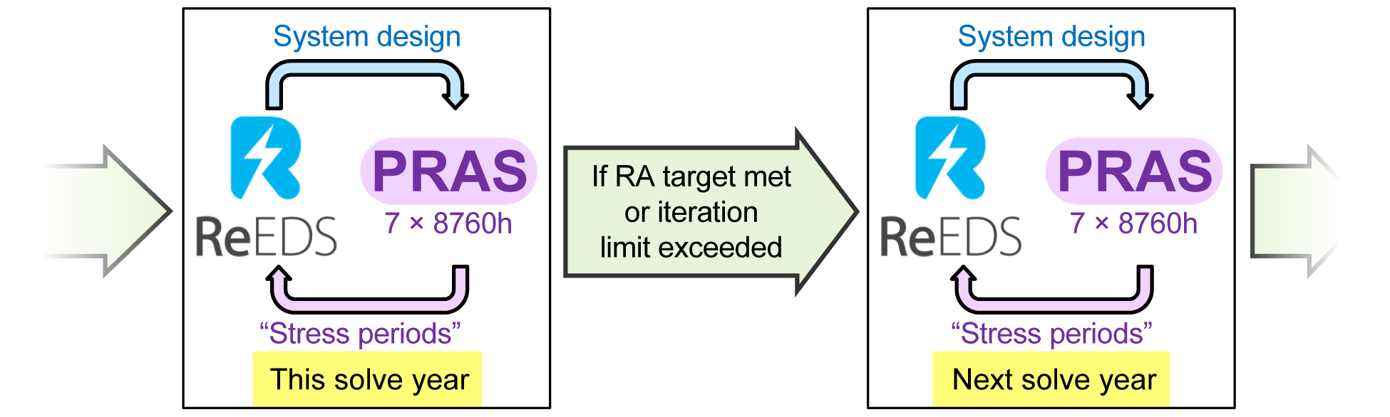
Fig. 17 Schematic illustrating the iteration between ReEDS and PRAS in each model year.
Model Formulation
ReEDS uses a linear program that governs the evolution and operation of the generation and transmission system. It seeks to minimize power sector costs as it makes various operational and investment decisions, subject to a set of constraints on those decisions.
The objective function is a minimization of both capital and operating costs for the U.S. electric sector, including the following:
The present value of the cost of adding or upgrading new generation, storage, and transmission capacity (including project financing)
The present value of operating expenses over the evaluation period[2] (e.g., expenditures for fuel and operations and maintenance [O&M]) for all installed capacity
The cost of several categories of ancillary services and storage
The cost of production technologies (e.g., hydrogen), direct air capture, and CO2 pipelines and storage
The cost of water access (if water resource constraints are active)
The cost or incentive applied by any policies that directly charge or credit generation or capacity
Penalties for rapid capacity growth as a proxy for manufacturing, supply chain, and siting/permitting limitations.
By minimizing these costs and meeting the system constraints (discussed below), the linear program determines the types of new capacity to construct (and existing capacity to retire) in each region during each model year to minimize systemwide cost. Simultaneously, the linear program determines how generation and storage capacity should be dispatched to provide the necessary grid services for all periods. The capacity factor for each technology, therefore, is an output of the model and not an input assumption.
The constraints that govern how ReEDS builds and operates capacity fall into several main categories:
Load balance constraints: Sufficient power must be generated within or imported by the transmission system to meet the projected load in each of the model zones in each of time steps during representative periods.
Resource adequacy constraints: Resource adequacy is a component of reliability that ensures sufficient available capacity to meet forecasted demand in all hours while accounting for outages and demand forecast errors. Constraints to meet resource adequacy requirements are applied during the “stress periods” and based on the linkage between ReEDS and PRAS as described in the Resource Adequacy section.
Operating reserve constraints: For shorter timescales, unexpected changes in generation and load are handled by the operating reserve requirements, which are applied for each reserve-sharing group (Operational Reliability). ReEDS can account for the following operating reserve requirements: regulation reserves, spinning reserves, and flexibility reserves.
Generator operating constraints: Technology-specific constraints bound the minimum and maximum power production and capacity commitment based on physical limitations and assumed average outage rates.
Transmission constraints: Power transfers among regions are constrained by the carrying capacity of transmission interfaces that connect the regions. Transmission constraints also apply to reserve sharing. A detailed description of the transmission constraints can be found in Transmission.
Resource constraints: Many renewable technologies, including wind, solar, geothermal, biopower, and hydropower, are spatially heterogeneous and constrained by the quantity available at each location. Several of the technologies include cost- and resource-quality considerations in resource supply curves to account for depletion, transmission, and competition effects. The resource assessments that seed the supply curves come from various sources; these are discussed in Generation and Storage Technologies, where characteristics of each technology are also provided. CO2 sequestration and water resource constraints are also represented.
Emissions constraints: ReEDS can limit or cap the emissions from fossil-fueled generators for sulfur dioxide (SO2), nitrogen oxide (NOx), carbon dioxide (CO2), and carbon dioxide-equivalent (CO2e), which includes CO2, CH4, and N2O. The emission limit and the emission per megawatt-hour by fuel and plant type are inputs to the model. Negative emissions are allowed using biomass with carbon capture and storage (BECCS) or direct air capture (DAC), and the emission constraint is based on net emissions. Emissions can be capped or taxed, with flexibility for applying either. Alternatively, emissions intensities can also be limited to certain bounds in ReEDS. The emissions constraints can be applied to stack emissions, or can be based on CO2 equivalent emissions, with the latter including upstream emissions and emissions from upstream methane leakage (see the Air Pollution section).[3] Methane leakage rates are input by the user.
Renewable portfolio standards or clean electricity standards: ReEDS can represent renewable portfolio standards (RPSs) and clean electricity standards constraints at the national and state levels. All renewable generation is considered eligible under a national RPS requirement. The renewable generation sources include hydropower, wind, CSP, geothermal, photovoltaics (PV), and biopower (including the biomass fraction of cofiring plants). The eligibility of technologies for state RPSs depends on the state’s specific requirements and thus varies by state. RPS targets over time are based on an externally defined profile. Penalties for noncompliance can be imposed for each megawatt-hour shortfall occurring in the country or a given state. In the same way, a clean energy standard constraint can be implemented to include nonrenewable low-emissions energy resources, such as nuclear and fossil fuels with carbon capture and storage (CCS) (Clean Energy Standards).
Spatial Resolution
ReEDS is typically used to study the CONUS.[4] Within the CONUS, ReEDS uses 134 regions for input data but by default runs the model using 132 regions (with region p119 aggregated into p122 and region p30 aggregated into p28). ReEDS model regions can be seen in Fig. 18. The model zones comprise groups of counties and do not align perfectly with real balancing authority areas. The zones respect state boundaries, allowing the model to represent individual state regulations and incentives. Transmission flows across the roughly 300 interfaces between model zones are subject to transfer limits, as discussed in the Transmission section. Additional geographical layers used to define model characteristics include 3 synchronous interconnections, 18 planning subregions designed after existing regional transmission organizations (RTOs), 13 North American Electric Reliability Corporation (NERC) reliability subregions, 9 census divisions as defined by the U.S. Census Bureau, and 48 states.[5] The spatial configuration in the model is flexible so the model can be run at various resolutions (i.e., aggregations of model zones), and data within the model are filtered to include data only for the regions being modeled in a given scenario.
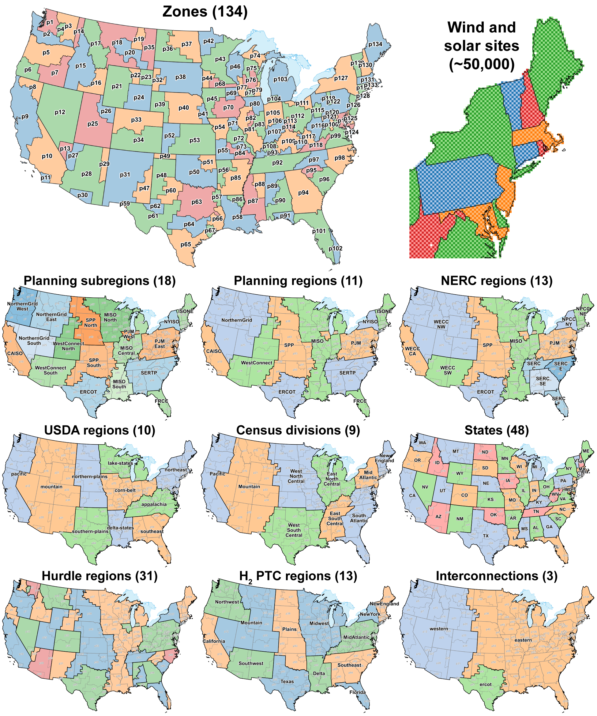
Fig. 18 Levels of spatial resolution used in ReEDS.
For more information on the spatial flexibility in the model, including running the model at county resolution, see Spatial Resolution Capabilities.
Temporal Resolution
Temporal inputs to ReEDS, including renewable energy capacity factors, electricity demand, and air temperature, are available at hourly (or finer) resolution across many weather years [Mai et al., 2022, National Renewable Energy Laboratory, 2024, National Renewable Energy Laboratory, 2024]. Given the high spatial resolution, large number of technologies, and multidecadal time horizon used in ReEDS, these temporal inputs—and the temporal resolution used within the linear optimization—must be simplified to achieve a tractable model size. Two methods of time series aggregation are combined in ReEDS:
A reduced number of representative periods (33 days by default) is selected and weighted to minimize deviation in regional wind and solar capacity factors and electricity demand between the weighted representative periods and complete time series.
Within the representative periods, hours are combined into chunks (of 3-hour duration by default), with operational constraints (such as chronological energy balancing for storage) acting on the aggregated chunks.
ReEDs allows 1-day or 5-day periods, with 1-day periods used by default (“periods” and “days” are hereafter used interchangeably). Fig. 19 and Fig. 20 provide two equivalent visualizations of modeled system dispatch in ReEDS: Fig. 19 shows the 3-hour national dispatch stack for the 33 representative periods, sorted by period weight; Fig. 20 shows the same dispatch stack, with each actual day mapped to its corresponding representative day.
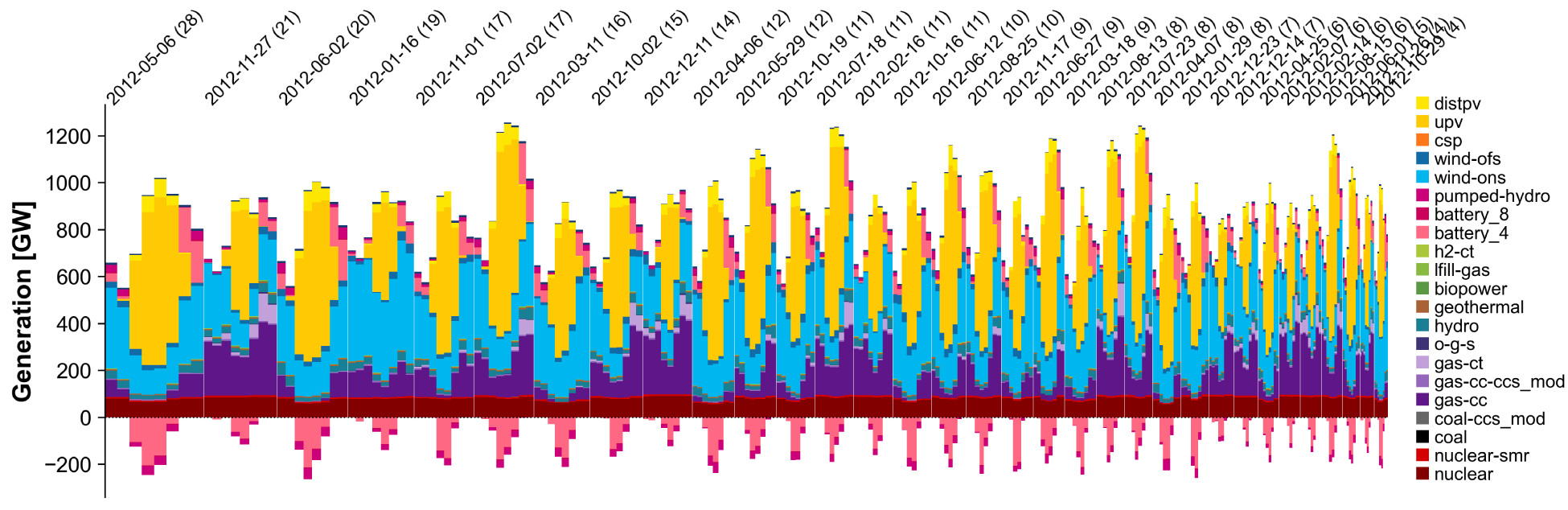
Fig. 19 National dispatch stack for an illustrative ReEDS scenario, organized by representative period (here, days). The width of each day is proportional to its weight—i.e., the number of days it is used to represent. Technologies are described in the generation and storage technologies section; the same color scheme is used throughout this documentation.

Fig. 20 National dispatch stack for an illustrative ReEDS scenario (the same scenario as in Fig. 19), organized by month of the year. Representative periods (here, days) are highlighted by dashed boxes. Each other day is represented by the representative day noted by the label in the upper left corner of the day. For example, December 1 is represented by the 27th representative day, which is November 1. The dispatch for each day represented by a given representative day is the same. (Dispatch is simulated within each of the model zones but is here aggregated to a national profile in postprocessing for visualization.)
Representative periods
Various methods are used for representative period selection in the literature (reviewed, for example, by [Teichgraeber and Brandt, 2022]). ReEDS includes options based on hierarchical clustering, k-means and k-medoids clustering, and an interregional optimization approach described by [Brown et al., 2025]. The optimization approach is used by default and is briefly described here.
The optimized method considers three “features” (wind capacity factor, solar capacity factor, and electricity demand) and their daily average values over a user-specified number of regions. The 18 planning subregions shown in Fig. 18 are used by default, resulting in 3 × 18 = 54 combinations of features and regions. The two-step optimization method is illustrated graphically in Fig. 21. First, a linear optimization is performed to identify a set of daily “weights” that, when multiplied by the observed daily feature values in each region and summed over the year, minimizes the error in weighted average regional feature values compared to their full-year values (Fig. 21a). The weights are truncated to a user-specified number of representative days (35 in this example), then rescaled and rounded to integers (Fig. 21b), giving the number of times each representative day is to be used over the modeled weather year(s). (In this example, December 23 is used 29 times, September 8 is used 3 times, and so on.)
Because some aspects of system operations are modeled with interday constraints (discussed below), each actual day must then be mapped to one of the modeled representative days, allowing a reconstructed chronological representation of the year (Fig. 21c). This mapping is performed in a second optimization, formulated as a mixed integer/linear problem (MILP), to minimize the sum of absolute differences between each day’s actual regional feature values and the feature values on the representative day to which it is mapped.
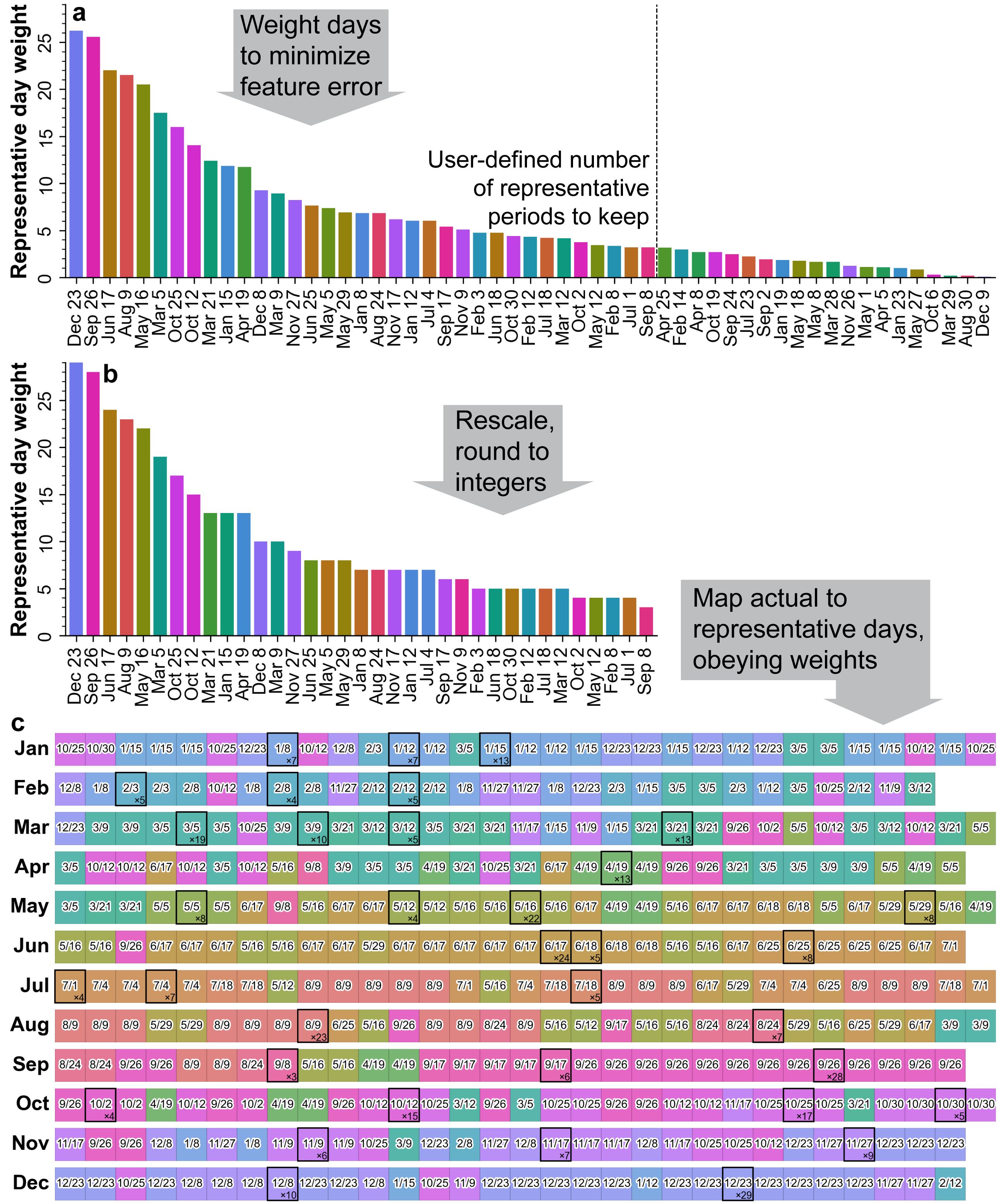
Fig. 21 Weighting and mapping of representative periods (here, days) in the optimized method. Reproduced from [Brown et al., 2025]. a, Identification and weighting of representative days to minimize errors in regional features (wind/solar capacity factor and electricity demand). b, Truncation to user-defined number of representative days, following by scaling and rounding of day weights to integers. c, Mapping of actual days to representative days, minimizing the sum of daily errors in regional feature values. Each day is labeled in month/day format by the representative day it is represented by; for days where the representative day coincides with the actual day, the day is surrounded by a black box and the value in the lower right corner indicates the weight of the representative day (i.e., the number of times it is used throughout the year), matching the value in b. This example uses the 2012 weather year, but the method can also be applied across multiple weather years.
Although the optimized method produces lower regional errors in wind and solar capacity factors and electricity demand than hierarchical clustering methods [Brown et al., 2025], time series aggregation always introduces some error through loss of resolution. Fig. 22 shows the regional error in wind capacity factor for an illustrative ReEDS scenario using 33 representative days. Regional errors can be reduced by using a larger number of representative periods at the expense of increased runtime.
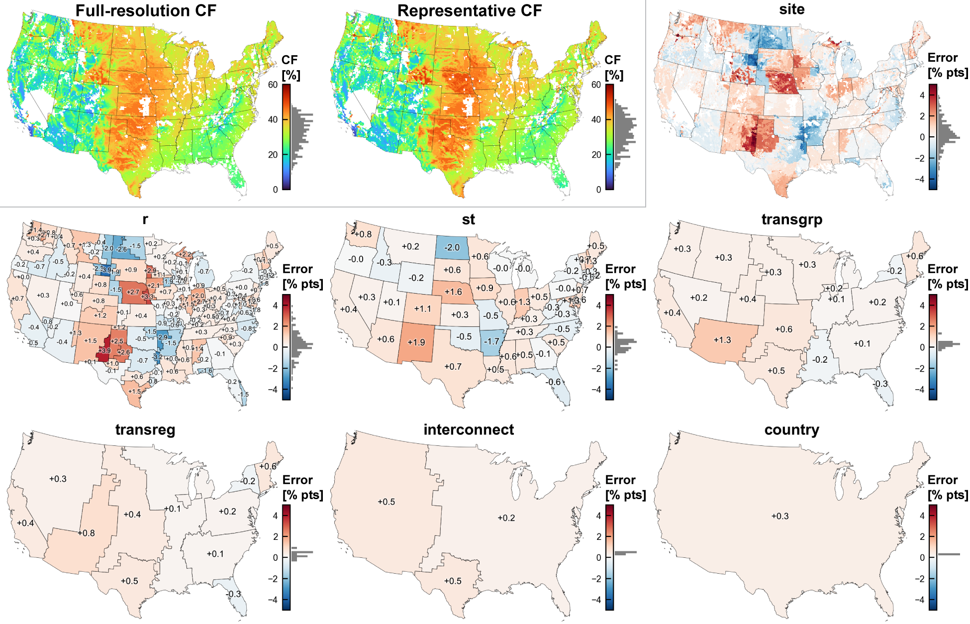
Fig. 22 Absolute wind capacity factor for full time resolution and representative periods (upper left) and error in wind capacity factor for representative periods relative to full time resolution, shown for different spatial resolutions in absolute percentage points (rest of figure). These results are for an illustrative ReEDS scenario using 33 representative days.
Weather years
ReEDS distinguishes between future model years (also referred to as solve years) during which operations and investments are optimized and weather years associated with hourly capacity factor and electricity demand profiles. These sets of years are entirely independent: Multiple weather years are used for resource adequacy calculations in each model year (for example, the modeled capacity mix in 2030 may be assessed against 2007–2013 weather), and the weather years are held fixed for each model year (so the 2030 and 2050 model years may both use 2007–2013 weather years for resource adequacy calculations).
Weather years are used differently for representative periods and resource adequacy calculations. By default, representative periods are drawn from the single 2012 weather year, whereas resource adequacy calculations use the 7 weather years spanning 2007–2013. The default 2007–2013 weather years are defined by the temporal scope of the Wind Integration National Dataset (WIND) Toolkit [National Renewable Energy Laboratory, 2024], which is used to calculate hourly wind capacity factors. Alternative weather profiles may be provided by the user, but the allowable weather years are constrained by the need for coincident hourly profiles for PV and wind capacity factors, electricity demand, and surface air temperature (used in the calculation of outage rates) for all model zones. The hourly wind and solar datasets in ReEDS include profiles for weather years 2007–2013 and 2016–2023. Historical hourly electricity profiles are also included for the same set of weather years.
Weather year settings
GSw_HourlyWeatherYears(default2012): Weather years from which to select representative periods, as described aboveresource_adequacy_years(default2007_2008_2009_2010_2011_2012_2013): Weather years to include in resource adequacy calculations
Interperiod linkages
Most operational constraints and costs are enforced either within individual representative periods (e.g., storage energy levels for batteries and pumped hydro are by default modeled with periodic boundary conditions wrapping from the end to the beginning of each period) or across all representative periods (e.g., renewable portfolio standards) without consideration of the chronological ordering of periods illustrated in Fig. 21c. Two model features—interperiod (or “long duration”) energy storage via hydrogen and generator startup costs—require consideration of interperiod chronology.
Hydrogen storage
Interperiod storage is modeled using assumptions consistent with gas-phase hydrogen (H2). Technical assumptions for H2 are described in the Hydrogen section. The temporal behavior of H2 production, storage, and use is illustrated in Fig. 23. Hydrogen production, storage injection/withdrawal, and consumption in hydrogen-fired turbines (with production and storage injection playing the role of “charging” and withdrawal and turbine consumption playing the role of “discharging”) are modeled using the same representative-period resolution (by default, 33 representative days) used for other operational variables, but the hydrogen reservoir level is modeled using actual periods (365 days in a single weather year by default). Consecutive runs of “charging” days add to the reservoir level over time, whereas runs of “discharging” days deplete it.
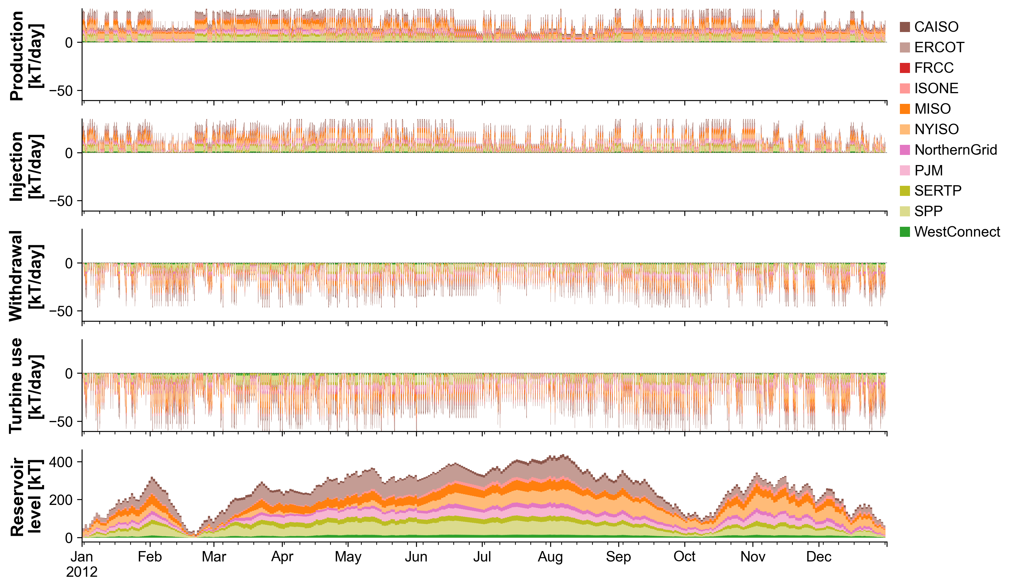
Fig. 23 Regional profiles for H2 production, storage injection, storage withdrawal, use in H2-CT turbines, and reservoir storage level over the course of a modeled year for an illustrative high-H2 scenario.
Temporal resolution for H2 storage
Two switches control the temporal behavior of H2 storage:
GSw_H2_StorTimestep(default1): Resolution at which to model H2 storage reservoir level. If set to1, storage level is resolved by period (typically single days, controlled by theGSw_HourlyTypeswitch). If set to2, storage level is resolved by time chunk (typically 3-hour chunks, controlled by theGSw_HourlyChunkLengthRepswitch).GSw_HourlyWeatherYears(default2012): Weather years from which to select representative periods, as described above. If set to multiple_-delimited years, H2 storage levels are modeled chronologically across all the specified years.
Unit commitment approximations
As a linear optimization problem, ReEDS does not directly model unit commitment. For a subset of technologies for which unit startup costs are expected to significantly affect aggregate fleetwide operations, two approximation methods are used by default:
Nuclear generation technologies are modeled with a fixed minimum generation level, set to 70% for conventional nuclear and 40% for small modular reactors (SMRs). (Forced and scheduled outages, discussed in the Outage rates section, still occur and are not subject to the minimum-generation constraint.)
For coal and CCS (both gas-CCS and coal-CCS), a linearized startup cost is applied based on the difference in dispatched generation between each pair of consecutive time chunks, including pairs of time chunks between different actual (not representative) periods. For example, in Fig. 21c, the 6/18 representative day has a weight of 5 and is followed by another 6/18 representative day three times, by 5/5 one time, and by 5/16 one time. Ramps between the first and second time chunk of 6/18 are thus counted 5 times; ramps from the last time chunk of 6/18 to the first time chunk of 6/18 are counted three times, ramps from the last time chunk of 6/18 to the first time chunk of 5/5 are weighted one time, and so on.
Fig. 24 illustrates how the minimum-generation constraint and linearized startup costs smooth out the generation profiles of the affected technologies.
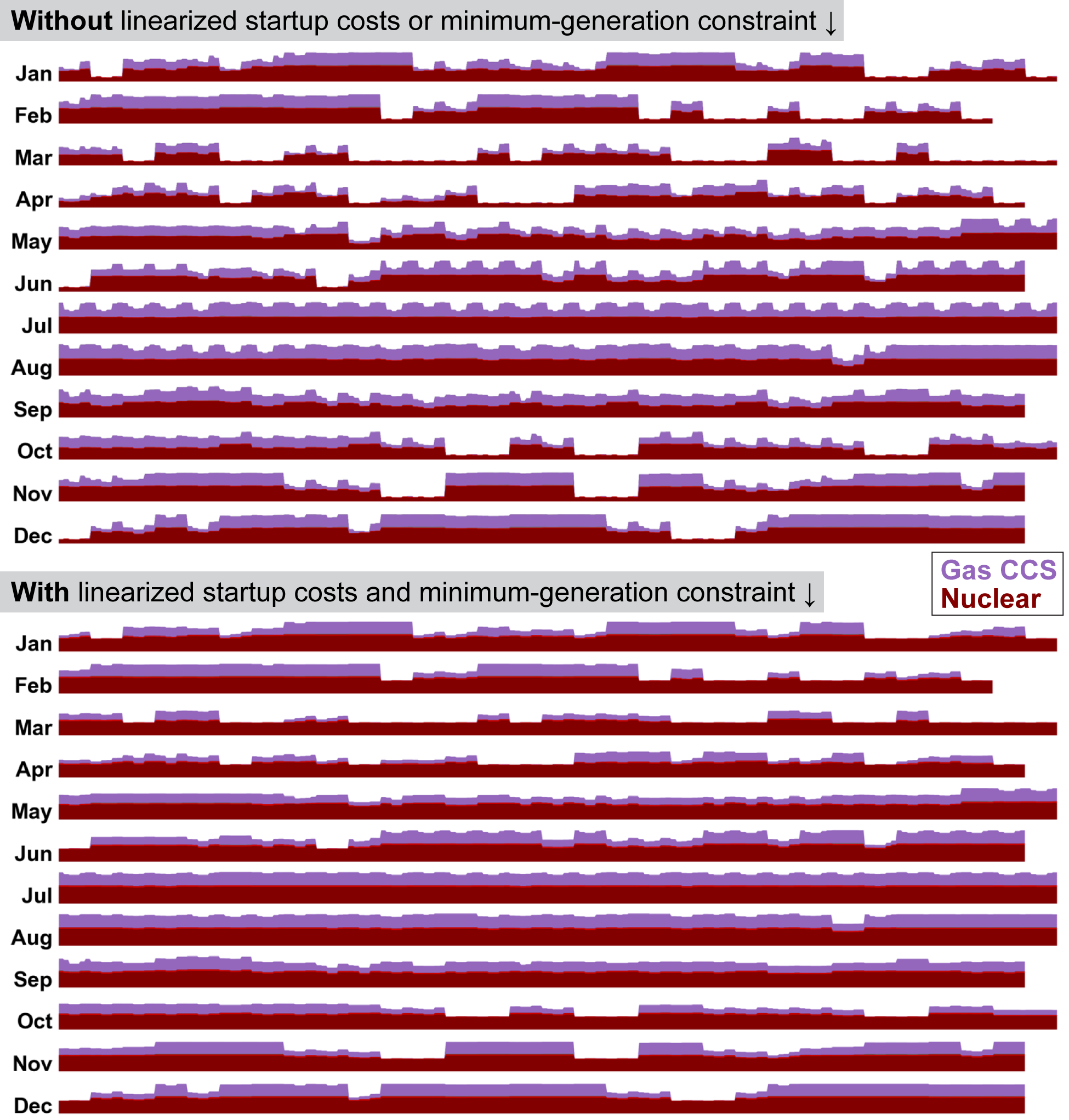
Fig. 24 Example national dispatch profiles for gas CCS and nuclear in illustrative low-carbon scenarios without (top) and with (bottom) linearized startup costs for gas CCS and a minimum-generation constraint for nuclear.
Unit startup considerations
Two switches control unit startup considerations:
GSw_MingenFixed(default1): Turn on (if1) or off (if0) the minimum generation constraint for the technologies included ininputs/plant_characteristics/mingen_fixed.csv(affects only nuclear by default).GSw_StartCost(default3): Specifies generation technologies for which to apply startup costs. The default setting of3specifies coal and CCS (leaving out nuclear, which is handled byGSw_MingenFixed). Startup costs are found atinputs/plant_characteristics/startcost.csv.
Generation and Storage Technologies
This section describes the electricity generating technologies included in ReEDS. Cost and performance assumptions for these technologies are not included in this report but are taken directly from the 2024 Annual Technology Baseline (ATB) [NREL, 2024] for all generation and storage technologies except BECCS (see Biopower).
Fossil and Nuclear Technologies
ReEDS includes all major categories of fossil (coal, gas, or oil) and nuclear generation technologies within its operating fleet and investment choices. Coal technologies are subdivided into pulverized and gasified (IGCC) categories, with the pulverized plants further distinguished by whether SO2 scrubbers are installed and whether their vintage[6] is pre- or post-1995. Pulverized coal plants have the option of adding a second fuel feed for biomass (this option is turned off by default). New coal plants can be added with or without CCS technology. Existing coal units built after 1995 with SO2 scrubbers installed also have the option of retrofitting CCS capability.
Natural gas generators are categorized as combustion turbine (CT), combined cycle (CC), or gas-CC with CCS.[7] The natural gas technologies all use the F-frame turbine cost and performance projections from the ATB, with gas-CC using the 2-on-1 configuration and the gas-CC with CCS using the 95% CCS capture projections.
There are also two types of nuclear (steam) generators: conventional and SMR. The conventional reactors draw their cost and performance from the “large” plants in the ATB and the SMRs from the “small” plants.
Finally, ReEDS includes landfill gas generators[8] and oil/gas steam generators, although these two technologies are not offered as options for new construction other than those already under construction. The model distinguishes each fossil and nuclear technology by costs, efficiency, and operational constraints.
Fossil and nuclear technologies are characterized by the following parameters:
Capital cost ($/MW)
Fixed and variable operating costs (dollars per megawatt-hour [$/MWh])
Fuel costs ($/MMBtu)
Heat rate (MMBtu/MWh)
Construction period (years) and expenses
Equipment lifetime (years)
Financing costs (such as interest rate, loan period, debt fraction, and debt-service-coverage ratio)
Tax credits (investment or production)
Minimum turndown ratio (%)
Ramp rate (fraction per minute)
Startup cost ($/MW)
Scheduled and forced outage rates (%).
Cost and performance assumptions for all new fossil and nuclear technologies are taken from the ATB [NREL, 2024] with options to use the Conservative, Moderate, or Advanced trajectories. Regional variations and adjustments are included and described in the Hydrogen section. Fixed operation and maintenance costs for coal plants increase over time with the plant’s age. Fixed operation and maintenance costs for nuclear plants increase by a fixed amount after 50 years of being online. These escalation factors are taken from the Annual Energy Outlook 2025 [EIA, 2025].
In addition to the performance parameters listed above, technologies are differentiated by their ability to provide operating reserves. In general, natural gas plants—especially combustion turbines—are better suited for ramping and reserve provision, whereas coal and large-scale nuclear plants are typically designed for steady operation. See Operational Reliability for more details.
The existing fleet of generators in ReEDS is taken from the National Energy Modeling System (NEMS) unit database from AEO2023 [EIA, 2025], with data supplemented from the March 2024 EIA 860M. In particular, ReEDS uses the net summer capacity, net winter capacity,[9] location, heat rate, variable O&M (VOM), and FOM to characterize the existing fleet. ReEDS uses a modified “average” heat rate for any builds occurring after 2010: A technology-specific increase on the full-load heat rate is applied to accommodate units not always operating at their design point. The modifiers, shown in Table 2, are based on the relationship between the reported heat rate in the ATB and the actual observed heat rate, calculated on a fleetwide basis for each fuel type.
Technology |
Adjustment Factor |
|---|---|
Coal (all) |
1.066 |
Gas-CC |
1.076 |
Gas-CT |
1.039 |
OGS |
0.875 |
Emissions rates from fuel-consuming plants are a function of the fuel emission rate and the plant heat rate. Burner-tip emissions rates are shown in Table 3. Because ReEDS does not differentiate coal fuel types, the coal CO2 emissions rate in the model is the average of the bituminous and subbituminous emissions rates from EIA.
Generator |
SO2 Emissions Rate |
NOx Emissions Rate |
CO2 Emissions Rate |
|---|---|---|---|
Gas-CT |
0.0098 |
0.15 |
117.00 |
Gas-CC |
0.0033 |
0.02 |
117.00 |
Gas-CC-CCS |
0.0033 |
0.02 |
11.70 |
Pulverized Coal with Scrubbers (pre-1995) |
0.2 |
0.19 |
210.55 |
Pulverized Coal with Scrubbers (post-1995) |
0.1 |
0.08 |
210.55 |
Pulverized Coal without Scrubbers |
1.11 |
0.19 |
210.55 |
IGCC Coal |
0.0555 |
0.085 |
210.55 |
Coal-CCS |
0.0555 |
0.085 |
21.06 |
Oil/Gas Steam |
0.299 |
0.1723 |
137.00 |
Nuclear |
0.0 |
0.0 |
0.0 |
Nuclear SMR |
0.0 |
0.0 |
0.0 |
Biopower |
0.08 |
0.0 |
0.0 |
a [EPA, 2008].
b The assumed CO2 pollutant rate for landfill gas is zero. However, ReEDS can track landfill gas emissions and the associated benefits as a postprocessing calculation. Landfill gas is assumed to have negative effective carbon emissions because the methane gas would otherwise be flared; therefore, it produces the less potent greenhouse gas.
ReEDS allows unabated gas-CC and coal plants to be retrofitted with CCS.
For existing plants, the cost of the upgrade and the performance changes are based on values from the NEMS unit database from AEO2025 [EIA, 2025].
For new plants, the upgrade cost is the difference between the CCS and non-CCS versions of the plant, and performance of the CCS plant adopts the CCS operating costs and characteristics.[10] For all CCS plant upgrades, there is also a capacity derate for plants that add CCS to represent the parasitic load of the CCS portion of the plant.
Upgraded capacity is allowed to operate for the number of years set by GSw_UpgradeLifeSpan, which may extend the lifetime of the plant beyond its regularly defined lifetime.
Upgraded CCS units are allowed to revert to their previous state in any solve year, which allows them to adopt their previous capacity and operating costs and characteristics.
Not all parameter data are given in this report.
For those values not included here, see the NREL ATB [NREL, 2024], or see the values in the ReEDS repository—particularly those in inputs/plant_characteristics.
Financing parameters and calculations are discussed in Capital Financing, System Costs, and Economic Metrics.
Renewable Energy Resources and Technologies
Renewable energy technologies modeled include land-based and offshore wind power, solar PV (both distributed and utility-scale), CSP with and without thermal storage, hydrothermal geothermal, near-field enhanced geothermal systems (EGS), deep EGS, run-of-the-river and reservoir hydropower (including upgrades and nonpowered dams), dedicated biomass, and cofired biomass technologies. Their characterization encompasses resource assessments,[11] projected technology improvements, grid interconnection costs, and operational implications of integration. The input assumptions, data sources, and treatments of these technologies are discussed in the following sections. Transmission considerations for renewable energy technologies are discussed in Interzonal Transmission.[12]
Biopower
ReEDS can generate electricity from biomass either in dedicated biomass integrated gasification combined cycle (IGCC) plants or cofired with coal in facilities that have been retrofitted with an auxiliary fuel feed. These cofire-ready coal plants can use biomass in place of coal to supply the fuel for up to 15% of the plant’s electricity generation. A cofire retrofit costs $305/kW (in 2017$) based on EIA’s Electricity Market Module assumptions [EIA, 2017, 101]. Cofiring is turned off by default in ReEDS but can be enabled if desired.
Dedicated and cofired plants source feedstock from the same biomass supply curves, which are derived from the Oak Ridge National Laboratory’s 2016 Billion-Ton Report [DOE, 2016]. Data from this report include estimates of biomass feedstock costs and total resource availability. Only woody biomass resources are allowed to be used for biopower plants; no other resource constraints are applied for nonrenewable energy technologies.
Fig. 25 illustrates the resource map and total supply curve by region as derived from [DOE, 2016] and used in ReEDS. Nationally, approximately 116 million dry tons of woody biomass are assumed to be available to the power sector. In addition to the supply curve price (which represents the cost of the resource in the field), ReEDS also assumes costs of $15 per dry ton for collection and harvesting as well as an additional $15 per dry ton for transport, based on estimates from a 2014 Idaho National Laboratory study [Jacobson et al., 2014]. Pathways with more limited biomass model the impact of a halving of the available resource and a doubling of collection, harvesting, and transport costs (58 million dry tons and $60 per ton), whereas the enhanced resource scenario models the opposite (doubling the available resource to 232 million dry tons and halving collection, harvesting, and transport costs to $15 per ton).
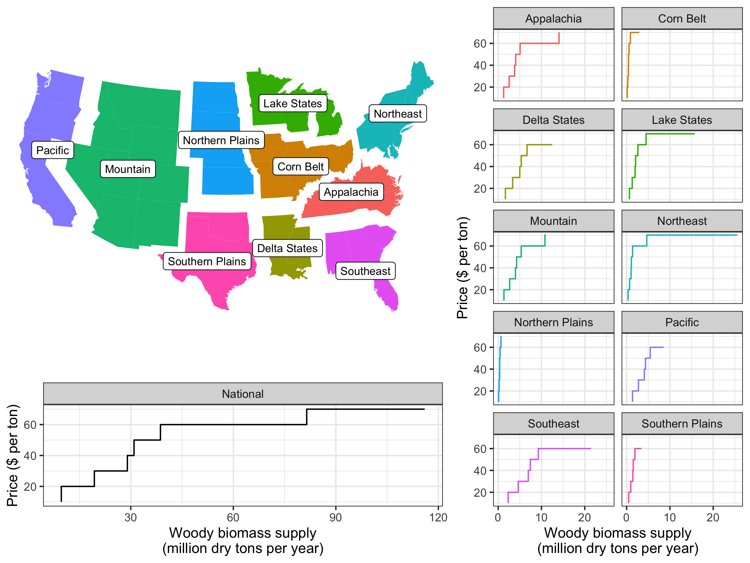
Fig. 25 Depiction of the regions used for the biomass supply curves (map, top left), based on U.S. Department of Agriculture regional divisions. The line plots to the right indicate the woody biomass supply curves for each region as used in ReEDS, as derived from data in [DOE, 2016]. The bottom-left plot summarizes the total national supply curve.
Because the model assumes zero life-cycle emissions for biomass, generation sources that use BECCS are assumed to have negative emissions. Table 4 summarizes cost and performance assumptions for BECCS plants. The uncontrolled emissions rate of woody biomass fuel is assumed to be 88.5 kilograms per million British thermal units (kg/MMBtu) [Bain et al., 2003]; after accounting for the heat rate of a BECCS plant and a 90% CCS capture rate, the negative emissions are approximately -1.22 to -1.11 tonnes/MWh of generation. Fuel consumed in BECCS plants is counted against the total biomass supply curve described above.
BECCS |
Capital Cost ($/kW) |
Variable O&M ($/kWh) |
Fixed O&M ($/kW-yr) |
Heat Rate (MMBtu/MWh) |
Emissions Rate (tonnes CO2/MWh) |
|---|---|---|---|---|---|
2020 |
5,580 |
16.6 |
162 |
15.295 |
-1.22 |
2035 |
5,333 |
16.6 |
162 |
14.554 |
-1.16 |
2050 |
5,100 |
16.6 |
162 |
13.861 |
-1.11 |
Concentrating Solar Power
Concentrating solar power (CSP) technology options in ReEDS encompass a subset of possible thermal system configurations, with and without thermal storage, as shown in Table 5. The various system types access the same resource potential, which is divided into 3–12 resource classes based on direct normal insolation (DNI), with three classes used by default. The CSP resource and technical potential are based on the latest version of NSRDB. Details of the CSP resource data and technology representation can be found in Appendix B of [Murphy et al., 2019]. By default, recirculating and dry cooling systems are allowed for future CSP plants getting built in ReEDS. Concentrating solar power cost and performance estimates are based on an assumed plant size of 100 MW.
Storage Duration (hours) |
Solar Multiple[13] |
Dispatchability |
Capacity Credit |
Curtailment |
|---|---|---|---|---|
None |
1.4 |
insolation-dependent |
Calculated based on hourly insolation |
Allowed |
6 |
1.0 |
dispatchable |
Calculated based on storage duration and hourly insolation |
Not allowed |
8 |
1.3 |
dispatchable |
Calculated based on storage duration and hourly insolation |
Not allowed |
10 |
2.4 |
dispatchable |
Calculated based on storage duration and hourly insolation |
Not allowed |
14 |
2.7 |
dispatchable |
Calculated based on storage duration and hourly insolation |
Not allowed |
The three default CSP resource classes are defined by power density of DNI, developable land area having been filtered based on land cover type, slope, and protected status. CSP resource in each region is represented by the same supply curve as UPV in (Solar Photovoltaics). Performance for each CSP resource class is developed using hourly resource data [Sengupta et al., 2018] from representative sites of each region. The weather files are processed through the CSP modules of the System Advisor Model (SAM) to develop performance characteristics for each CSP resource class and representative CSP system considered in ReEDS. Resources are then scaled in ReEDS by the ratio of the solar multiple of the CSP plant.
The representative CSP system without storage used to define system performance in ReEDS is a 100-MW trough system with an SM of 1.4. Because CSP systems without storage are nondispatchable, output capacity factors are defined directly from SAM results. The average annual capacity factors for the solar fields of these systems range from 20% (Class 1 resource) to 29% (Class 12 resource).
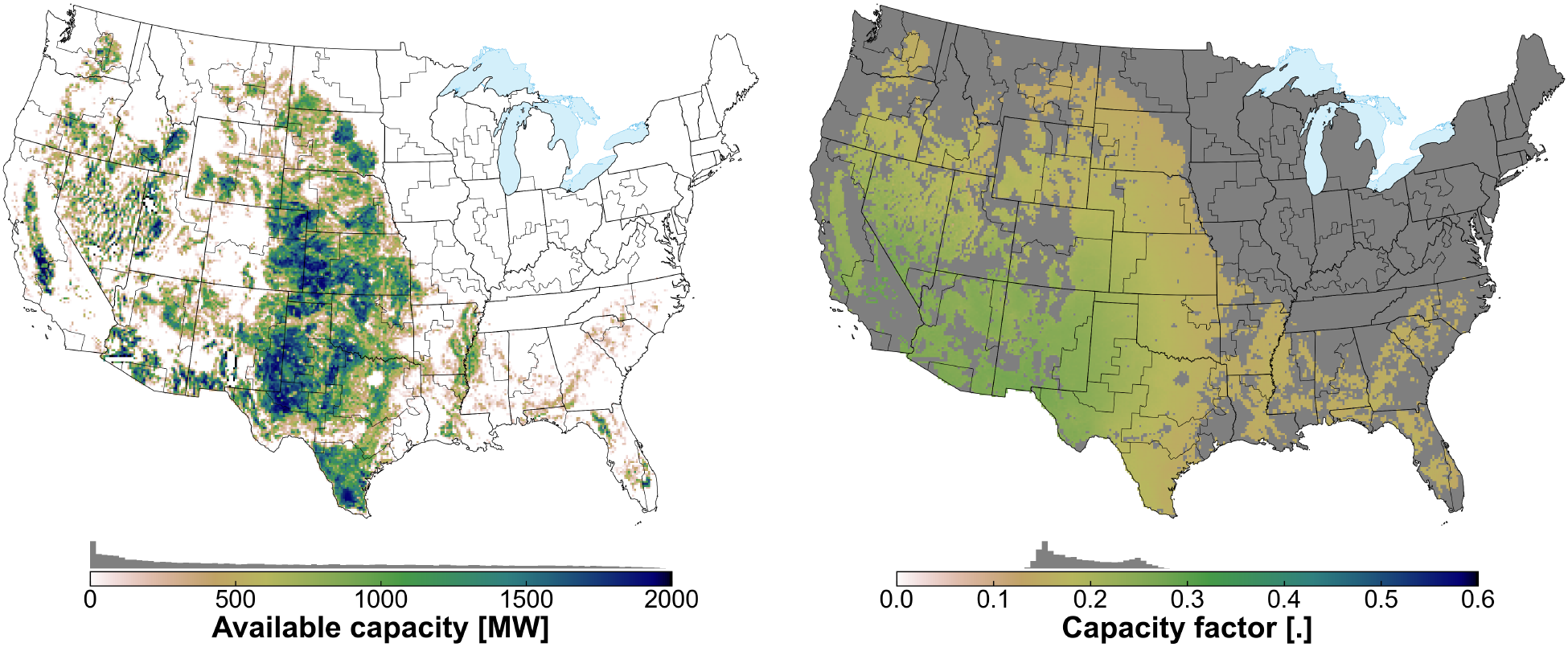
Fig. 26 CSP resource availability and solar field capacity factor for the CONUS.
The representative system for any new CSP with thermal energy storage is a tower-based configuration with a molten-salt heat-transfer fluid and a thermal storage tank between the heliostat array and the steam turbine.[14] Two CSP with storage configurations are available as shown in Table 5.
For CSP with storage, plant turbine capacity factors by time slice are an output of the model—not an input—because ReEDS can dispatch collected CSP energy independent of irradiation. Instead, the profiles of power input from the collectors (solar field) of the CSP plants are model inputs, based on SAM simulations from weather files.
CSP settings
New CSP deployment is turned off by default but can be enabled by setting the
GSw_CSPswitch to1.
Geothermal
The geothermal resource has two distinct subcategories in ReEDS:
The hydrothermal resource represents potential sites with appropriate geological characteristics for the extraction of heat energy. The hydrothermal potential included in the base supply curve comprises only identified sites, with a separate supply curve representing the undiscovered hydrothermal resource.
EGS sites are geothermal resources that have sufficient temperature but lack the natural permeability, in situ fluids, or both, to be hydrothermal systems. Developing these sites with water injection wells could create engineered geothermal reservoirs appropriate for harvesting heat.
EGS is further separated into near-field EGS and deep EGS based on proximity to known hydrothermal features. Near-field EGS represents additional geothermal resource available near hydrothermal fields that have been identified. Deep EGS represents available geothermal resource not tied to existing hydrothermal sites and at depths below 3.5 km.
Geothermal in ReEDS represents geothermal power production with representative size up to 100 megawatts electric (MWe). Geothermal resource classes are defined by reservoir temperature ranges, which are closely linked to the cost of a plant normalized by generation capacity. Energy conversion processes, including binary and flash cycles, are linked to reservoir temperature and are specified by resource class. Plants with reservoir temperatures <200°C (Class 7–10) use a binary cycle, which uses a heat exchanger and secondary working fluid with a lower boiling point to drive a turbine. All other reservoir temperatures assume a turbine is driven directly by working fluid from the geothermal wells. These assumptions are aligned with those in the 2024 ATB.
Table 6 lists the technical resource potential for the different geothermal categories.
Resource Class |
Reservoir Temperature (°C) |
Hydrothermal |
Near-Field EGS |
Deep EGS |
|---|---|---|---|---|
Class 1 |
> 325 |
- |
0.2 |
7.3 |
Class 2 |
300–325 |
2.2 |
0.2 |
35 |
Class 3 |
275–300 |
1.2 |
0.1 |
177 |
Class 4 |
250–275 |
0.7 |
0.1 |
1696 |
Class 5 |
225–250 |
0.2 |
0.1 |
4633 |
Class 6 |
200–225 |
0.9 |
0.2 |
6467 |
Class 7 |
175–200 |
12 |
0.3 |
3234 |
Class 8 |
150–175 |
342 |
0.3 |
- |
Class 9 |
125–150 |
2823 |
0.03 |
- |
Class 10 |
<125 |
699 |
- |
- |
Total |
3881 |
1.4 |
16249 |
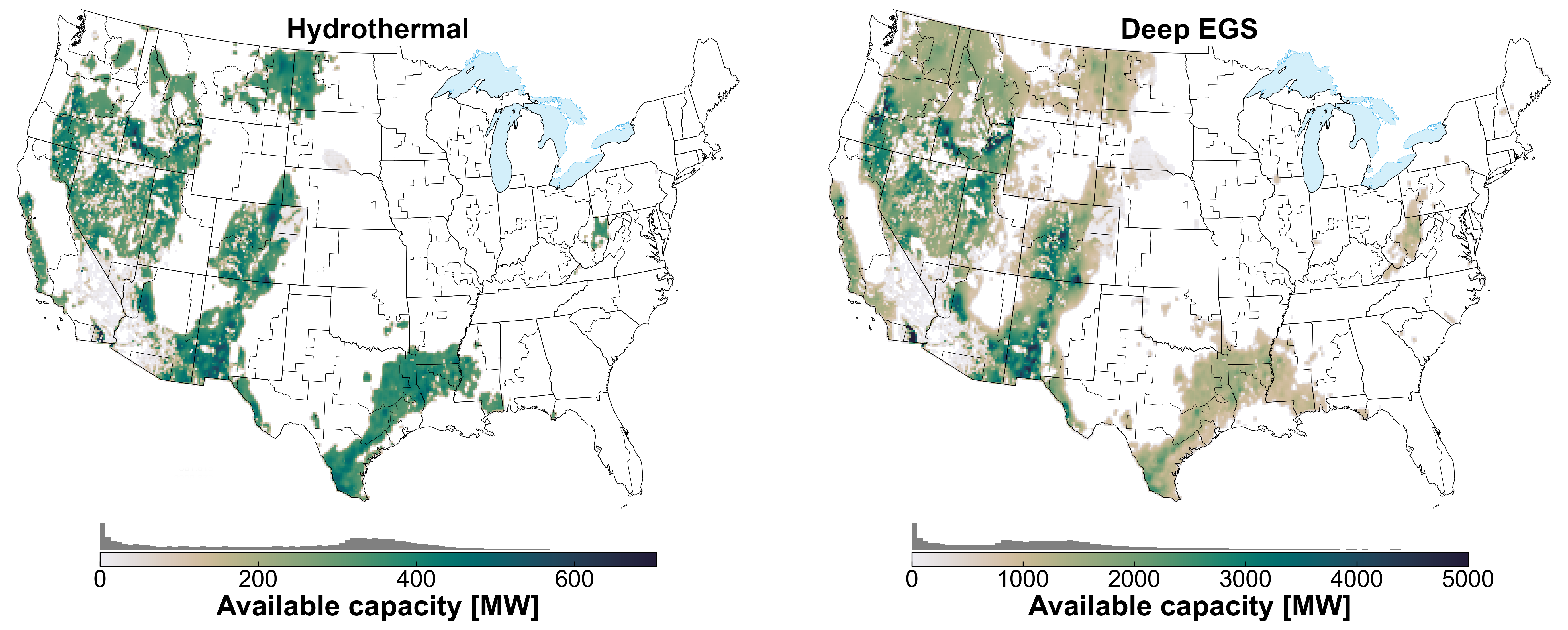
Fig. 27 Resource availability for hydrothermal (left) and deep EGS (right) for the CONUS.
The default geothermal resource assumptions allow for hydrothermal sites. Hydrothermal resources have a defined fraction, which is considered identified resources based on the U.S. Geological Survey’s 2008 geothermal resource assessment. The undiscovered portion of the hydrothermal resource is limited by a discovery rate defined as part of the GeoVision Study [DOE, 2019]. The geothermal supply curves are based on the analysis described by [Augustine et al., 2019] and are shown in Fig. 27. The hydrothermal and near-field EGS resource potential is derived from the U.S. Geological Survey’s 2008 geothermal resource assessment [Williams et al., 2008], whereas the deep EGS resource potential is based on an update of the EGS potential from the Massachusetts Institute of Technology [Tester et al., 2006]. As with other technologies, geothermal cost and performance projections are from the ATB [NREL, 2024]. Default geothermal capacity representation in ReEDS is categorized by depth and is based on reV analysis [Pinchuk, Paul and et al., 2023], which estimates potential and site-based levelized cost of energy (LCOE) based on resource assessment at various depths, development constraints, land use characteristics, and grid infrastructure (spur line transmission) costs. Although hydrothermal supply curves are based on a 3.5-km resource depth reV scenario, deep EGS supply curves are aggregated based on lowest total LCOE from different reV scenario depths ranging from 3.5 km to 6.5 km (most of the resource in Table 6 is at 6.5-km depth), highlighting the assumption that for EGS it is not possible to develop multiple resource depths simultaneously at a site.
Hydropower
The existing hydropower fleet representation is informed by historical performance data. From the nominal hydropower capacity in each zone, monthly capacity adjustments are used for Western Electricity Coordinating Council (WECC) regions based on data from the 2032 Anchor Data Set (ADS) [WECC, 2024]. Monthly capacity adjustments allow more realistic monthly variations in maximum capacity because of changes in water availability and operating constraints. These data are not available for non-WECC regions. Future energy availability for the existing fleet is defined using monthly plant-specific hydropower capacity factors averaged for 2010–2019 as reported by Oak Ridge National Laboratory HydroSource data (https://hydrosource.ornl.gov/datasets). Capacity factors for historical years are calibrated from the same data source so modeled generation matches historical generation. Pumped storage hydropower (PSH), both existing and new, is discussed in Storage Technologies.
Three categories of new hydropower resource potential are represented in the model:
Upgrade and expansion potential for existing hydropower
Potential for powering nonpowered dams (NPD)
New stream-reach development potential (NSD).
The supply curves for each are discussed in detail in the Hydropower Vision report [DOE, 2016], particularly Chapter 3 and Appendix B.
ReEDS does not currently distinguish between different types of hydropower upgrades, so upgrade potential is nominally represented generically as a potential for capacity growth that is assumed to have the same energy production potential per capacity (i.e., capacity factor) as the corresponding existing hydropower capacity in the region. An optional representation of hydropower upgrades decouples capacity and energy upgrades so the model can choose either type of upgrade independently. The quantity of available upgrades is derived from a combination of limited resource assessments and case studies by the U.S. Bureau of Reclamation Hydropower Modernization Initiative (HMI), U.S. Army Corps of Engineers, and National Hydropower Asset Assessment Program (NHAAP) Hydropower Advancement Project [Montgomery et al., 2009, Bureau of Reclamation, 2011]. Upgrade availability at federal facilities not included in the HMI is assumed to be the HMI average of 8% of the rated capacity, and upgrade availability at nonfederal facilities is assumed to be the NHAAP average of 10% of the rated capacity. Rather than making all upgrade potential available immediately, upgrade potential is made available over time at the earlier of either the Federal Energy Regulatory Commission (FERC) license expiration (if applicable) or the turbine age reaching 50 years. This feature better reflects institutional barriers and industry practices surrounding hydropower facility upgrades. The total upgrade potential from this methodology is 6.9 GW (27 terawatt-hours [TWh]/yr).
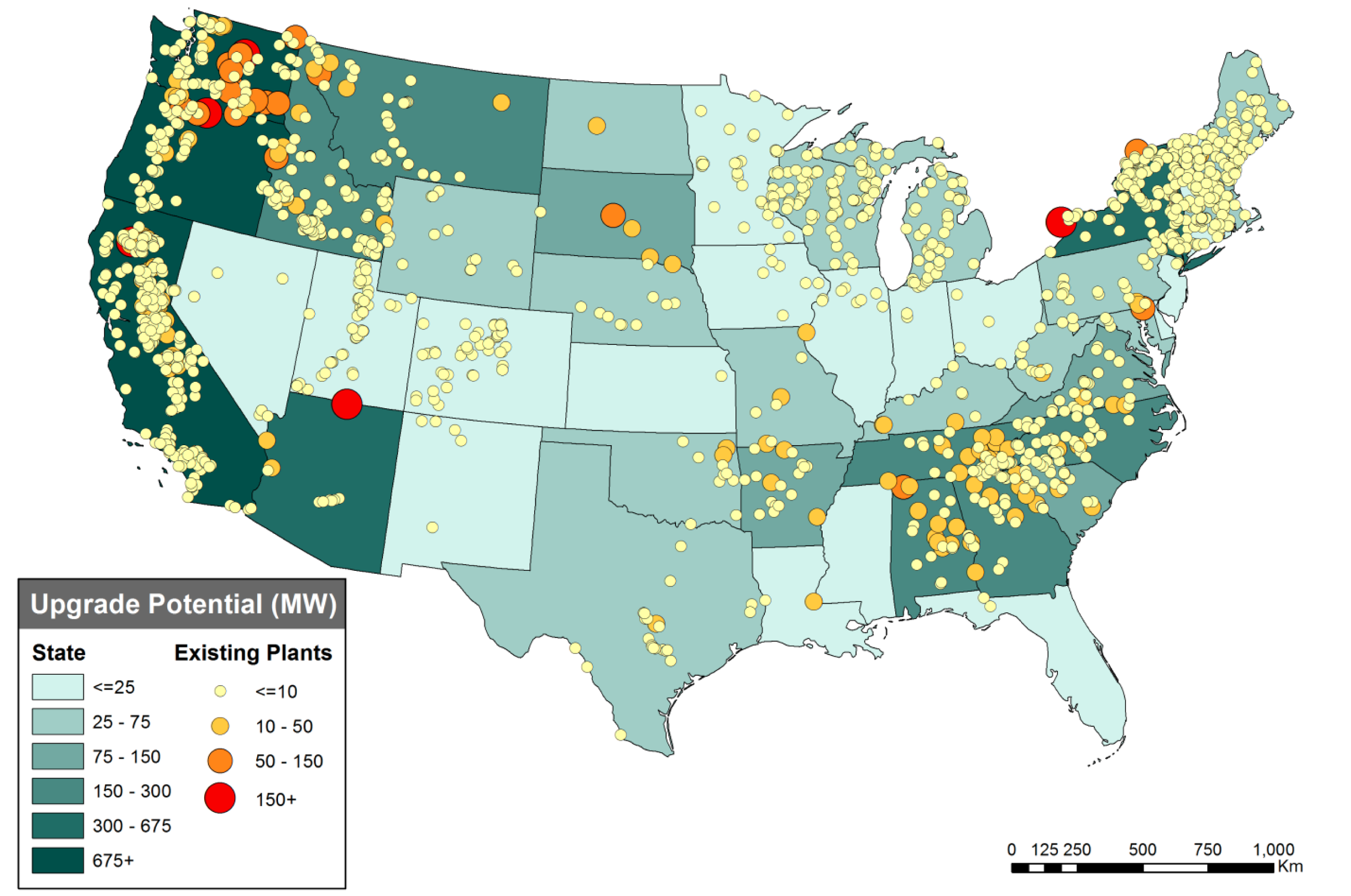
Fig. 28 Modeled hydropower upgrade resource potential [DOE, 2016].
NPD resource is derived from the 2012 NHAAP NPD resource assessment [Hadjerioua et al., 2013, Kao et al., 2014], where the modeled resource of 5.0 GW (27 TWh/yr) reflects an updated site sizing methodology, data corrections, and an exclusion of sites less than 500 kW to allow better model resolution for more economic sites.

Fig. 29 Modeled nonpowered dam resource potential [DOE, 2016].
NSD resource is based on the 2014 NHAAP NSD resource assessment [Kao et al., 2014], where the modeled resource of 30.7 GW (176 TWh/yr) reflects the same sizing methodology as NPD and a sub-1-MW site exclusion, again to improve model resolution for lower-cost resource. The NSD resource assumes “low head” sites inundating no more than the 100-year flood plain and excludes sites within areas statutorily barred from development—national parks, wild and scenic rivers, and wilderness areas.

Fig. 30 Modeled new stream-reach development resource potential [DOE, 2016].
The combined hydropower capacity coupled with the costs from the ATB [NREL, 2024] results in the supply curve shown in Fig. 30. If there is prescribed capacity from EIA unit data where insufficient capacity is available in the associated hydropower supply curve, capacity equal to the unavailable prescribed capacity is added to the supply curve at the cost of the lowest-cost bin.
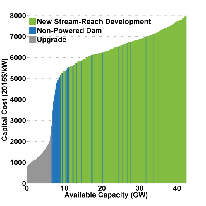
Fig. 31 National hydropower supply curve of capital cost versus cumulative capacity potential.
The hydropower operating parameters and constraints included in ReEDS do not fully reflect the complex set of operating constraints on hydropower in the real world. Detailed site-specific considerations involving a full set of water management challenges are not easily represented in a model with the scale and scope of ReEDS, but several available parameters allow a stylized representation of actual hydropower operating constraints [Stoll et al., 2017].
Each hydropower category can be differentiated into “dispatchable” or “nondispatchable” capacity, with “dispatchable” defined in ReEDS as the ability to provide the following services:
Diurnal load following within the capacity and average daily energy limits for each season
Planning (adequacy) reserves with full rated capacity
Operating reserves up to a specified fraction of rated capacity if the capacity is not currently being used for energy production.
“Nondispatchable” capacity, on the other hand, provides the following:
Constant energy output in each season so all available energy is used
Planning reserves equal to the output power for each season
No operating reserves.
Dispatchable capacity is also parameterized by a fractional minimum load, with the maximum fractional capacity available for operating reserves as 1 minus the fractional minimum load. The existing fleet and its corresponding upgrade potential are differentiated by dispatchability using data from the Oak Ridge National Laboratory Existing Hydropower Assets Plant Database (https://hydrosource.ornl.gov/dataset/EHA2023), which classifies plants by operating mode. Plants with operating modes labeled as Peaking, Intermediate Peaking, Run-of-River/Upstream Peaking, and Run-of-River/Peaking are classified as dispatchable in ReEDS, and plants with other operating modes are classified as nondispatchable. In total, 47% of existing capacity and 49% of upgrade potential is assumed nondispatchable. ReEDS also includes the option to enable hydroposwer upgrade pathways where existing nondispatchable hydropower can be upgraded to be dispatchable hydropower—or existing dispatchable hydropower can be upgraded to add pumping and become a pump-back hydropower facility. A pump-back facility is constrained similarly to a PSH facility except input energy can come from natural water inflows in addition to the grid. These upgrade options can be made available at a user-specified capital cost. Hydropower upgrades are unavailable by default because there is high uncertainty about where such upgrades are feasible, but these optional features allow users to explore the potential and value of increasing hydropower fleet flexibility, which is discussed in detail in [Cohen and Mowers, 2022].
The same WECC ADS database used to define intra-annual changes in maximum capacity is used to define region-specific fractional minimum capacity for dispatchable existing and upgraded hydropower in WECC [WECC, 2024]. Lacking minimum capacity data for non-WECC regions, 0.5 is chosen as a reasonable fractional minimum capacity.
Both the NPD and NSD resource assessments implicitly assume inflexible, run-of-river hydropower, so all NPD and NSD resource potential is assumed nondispatchable. Additional site-specific analysis could allow recategorizing portions of these resources as dispatchable, but 100% nondispatchable remains the default assumption.
Land-Based Wind
Land-based wind cost and performance assumptions are taken directly from ATB 2024 [NREL, 2024]. These inputs include capital costs, fixed O&M (FOM) costs, and average capacity factor improvements over time. Capacity factors for wind plants coming online from 2010 through 2023 are taken from the Land-Based Wind Market report [Wiser et al., 2023].
Available land-based wind resources and site-specific cost and performance are based on [Lopez et al., 2025], using outputs of the reV model [Maclaurin et al., 2021]. The Reference Access case includes more than 49,000 potential wind sites, totaling more than 9,400 gigawatts (GW). Limited Access and Open Access supply curves are also available. Available resource for the three access cases and associated average capacity factors are shown in Fig. 32. In ReEDS, each wind site is characterized with a supply curve cost, which comprises transmission spur line and reinforcement upgrade costs as well as site-specific capital cost adjustments based on region, land cost, and site capacity (to account for economies of scale). See Interzonal Transmission for more discussion of the interconnection supply curves for accessing the wind resource.
The individual wind sites are grouped into 10 resource classes based on k-means-based clustering of average annual capacity factors. Distinct wind generation profiles are represented in ReEDS for each region and class, based on capacity-weighted averages of all sites of that region and class. Sites are also grouped into a flexible number of supply curve cost bins in ReEDS, with 10 bins used by default for each ReEDS region and class.
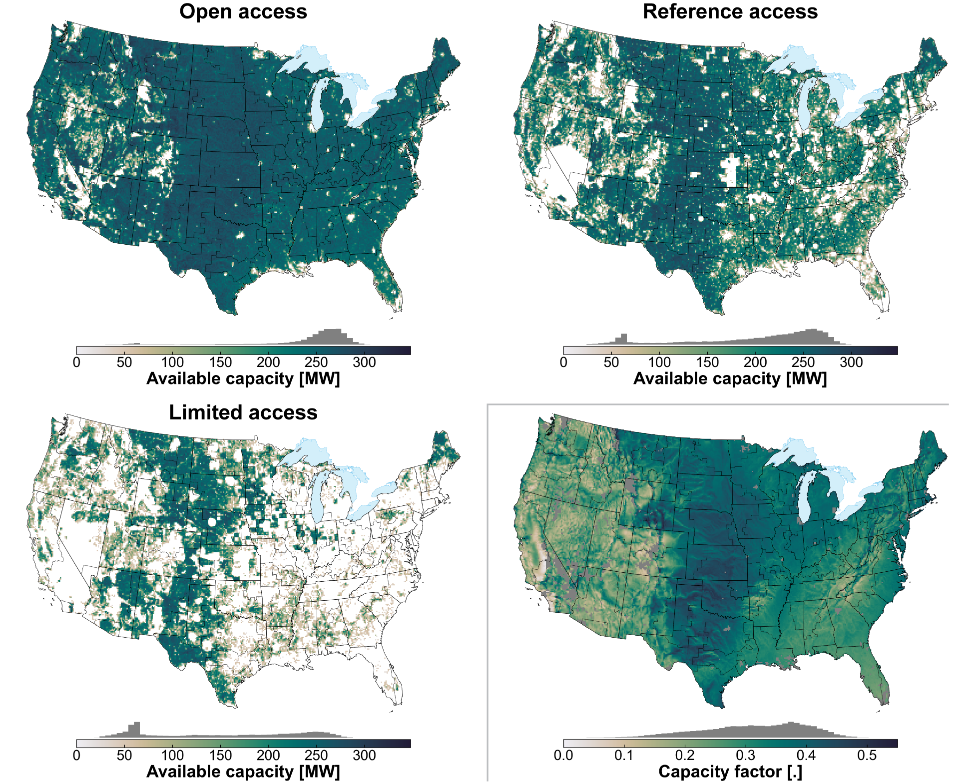
Fig. 32 Land-based wind resource availability and capacity factor for the three siting scenarios included in ReEDS.
Offshore Wind
ReEDS represents two offshore wind technologies: fixed and floating. Base cost and performance assumptions in ReEDS for the two technologies are based on one reference fixed offshore site in New York Bight and one reference floating offshore site in Humboldt County, California, including capital costs, FOM costs, and average capacity factor improvements over time.
There is substantial diversity in offshore wind generators, in distance from shore, water depth, and resource quality. ReEDS subdivides offshore wind potential into 10 resource classes: 5 each for fixed-bottom and floating turbine designs. Fixed-bottom offshore wind development is limited to resources <60 meters (m) in depth using either current technology monopile foundations (0–30 m) or jacket (truss-style) foundations (30–60 m). Offshore wind using a floating anchorage could be developed for greater depths and are assumed to be the only feasible technology for development for resource deeper than 60 m. Within each category, the classes are distinguished by resource quality; supply curves then differentiate resource by cost of accessing transmission in a similar fashion as land-based wind but using five cost bins per region and class.
Eligible offshore area for wind development includes open water within the U.S.-exclusive economic zone having a water depth less than 1,000 m, including the Great Lakes. As with land-based resource, offshore zones are filtered to remove areas considered unsuitable for development, including national marine sanctuaries, marine protected areas, wildlife refuges, shipping and towing lanes, offshore platforms, and ocean pipelines. The offshore technology selection is made using the Offshore Wind Cost Model, which selects the most economically feasible technology for developing a wind resource [Beiter and Stehly, 2016]. See also [Lopez et al., 2025] for more information on the development of the resource supply curves.
Resource availability varies across different siting access cases: The Reference Access case has 4,064 sites totaling 2.97 terawatts (TW), the Open Access case has 4,524 sites totaling 3.534 TW, and the Limited Access case with 3,166 sites totals 2.212 TW. Modeled site-level capacity factor and resource availability are shown in Fig. 33. Additional details regarding offshore wind resource modeling can be found in [Lopez et al., 2025].
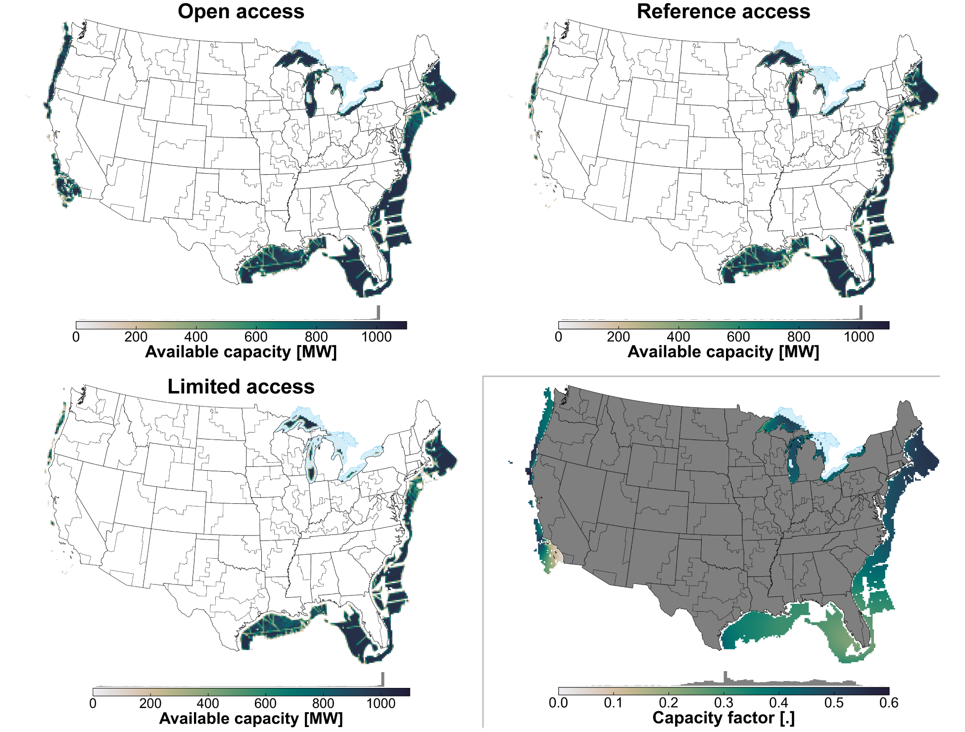
Fig. 33 Offshore wind resource availability by siting access case for the CONUS
Each wind site in a supply curve is characterized in ReEDS by a supply curve cost, which comprises capital adder and transmission adder costs. The capital adder incorporates the site-specific technology, regional differences, and economies of scale. Refer to [Shields et al., 2021] for details on how economies of scale impact the site capital cost. The transmission cost adder includes the array, export costs, and point of interconnection (POI)/substation, spur line, and reinforcement costs. The site capital cost adder is aggregated into region-bin-class to sync with the reference site “base” overnight capital cost from the ATB.
[IRS, 2023] defines the energy property and rules for investment tax credit (ITC) eligibility. In ReEDS, this translates into array, export cable, and substation/POI costs. However, for consistency in implementation with other technologies, because the components that are not eligible for the ITC (spur line and reinforcement) take up of only 22% of transmission costs, and transmission costs comprise only 30% of total cost, we decided to apply the ITC to all transmission cost components to make OSW format consistent with LBW (the extra error in applying the ITC to all transmission cost components versus to just the ITC eligible components is about 2%).
State offshore wind mandates are represented in accordance with [McCoy et al., 2024]. The 2020, 2030, 2040, and 2050 state-mandated capacity can be seen in Table 24. States not included in the table do not have any mandated offshore wind capacity.
Solar Photovoltaics
ReEDS differentiates among three solar PV technologies:
Large-scale utility PV (UPV)
Hybrid large-scale utility PV with battery (PVB)
Rooftop PV (distPV).
Investments in UPV and PVB are evaluated directly in ReEDS, whereas rooftop PV deployment and performance are exogenously specified as inputs into ReEDS based on results from the Distributed Generation Market Demand (dGen) model. PV capacity is tracked in megawatts direct current (MWDC) within the model but converted to megawatts alternating current (MWAC) in reported outputs.
Utility-scale PV
UPV represents utility-scale, single-axis-tracking PV systems with a representative size of 100 MWDC and an array density of 43 MWDC per square kilometer (km2) [Lopez et al., 2025]. An inverter loading ratio of 1.34 is assumed for utility-scale PV. Resource potential is assumed to be located on large parcels outside urban boundaries, excluding federally protected lands, inventoried roadless areas, U.S. Bureau of Land Management areas of critical environmental concern, areas of excessive slope, and other exclusions. ReEDS provides supply curves and profiles representing three siting exclusion scenarios: reference, limited, and open access.
Hourly generation profiles are simulated using NREL’s reV model [Maclaurin et al., 2019, National Renewable Energy Laboratory, 2024] at 11.5-km by 11.5-km resolution across the CONUS using irradiance data from the National Solar Radiation Database (NSRDB) [Sengupta et al., 2018, National Renewable Energy Laboratory, 2024]. Modeled capacity factor and siting availability are shown in Fig. 34.
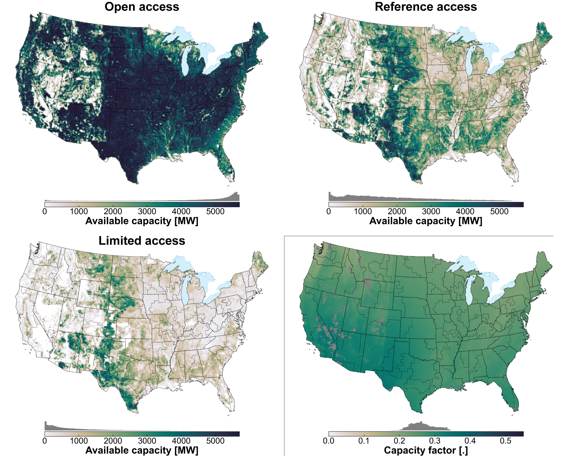
Fig. 34 UPV resource availability and DC capacity factor [MWACavailable/MWDCnameplate] for the open, reference, and limited siting access scenarios.
Site-level costs and capacity factor profiles are compiled into supply curves for each model zone. Within each zone, the PV supply curve is differentiated into five resource classes based on annual capacity factor. Each class is further differentiated by interconnection cost (described in Interzonal Transmission) across groups of reV sites.
The efficiency of installed PV capacity is assumed to degrade by 0.7%/year [NREL, 2024]. Additional details on the UPV configuration, siting exclusion criteria, profiles, and supply curve results are provided by [Lopez et al., 2025].
Utility-scale PV settings
Siting availability (reference, limited, or open) is controlled by the
GSw_SitingUPVswitchAnnual degradation is specified in the
inputs/degradation/degradation_annual.csvfileThe UPV ILR is specified by the
ilr_utilityparameter in theinputs/scalars.csvfile
PV + battery hybrids
For hybrid systems, the default technology represents a loosely DC-coupled system in which the PV and battery technologies share a bidirectional inverter and POI, and the battery can charge from either the coupled PV or the grid.
The PVB design characteristics can be user defined for up to three configurations, but the default configuration involves an inverter loading ratio of 2.2 (slightly higher than stand-alone PV) and a coupled battery with a preset duration, whose power-rated capacity is 50% of the inverter capacity.
The PVB duration default is 4 hours and can be adjusted using GSw_PVB_Dur.
The PVB investment option leverages the existing representations of the independent component technologies, but the cost and performance characteristics differ from the simple sum of the separate (PV and battery) parts. For example, the capital costs associated with the fully integrated PVB hybrid system are reduced based on the cost of a shared inverter and other balance-of-system components; as a result, the percentage savings vary by PVB configuration. Improved performance characteristics are captured through slightly enhanced battery round-trip efficiencies and explicit time series generation profiles; the latter enables a representation of the PVB system’s ability to divert otherwise clipped energy to the coupled battery (during periods when solar output exceeds the inverter capacity) and avoid curtailment.
Distributed PV
Rooftop PV includes commercial, industrial, and residential systems.
These systems are assumed to have an inverter loading ratio (ILR) of 1.1.
Existing rooftop PV capacities are obtained from U.S. Energy Information Administration (EIA)-861 data spanning 2010 to 2022 [EIA, 2024].
dGen, a consumer adoption model for the CONUS rooftop PV market, is used to develop future scenarios for rooftop PV capacity, including the capacity deployed by zone and the precurtailment energy production by that capacity [Sigrin et al., 2016].
The default dGen trajectories used in this version of ReEDS are based on the residential and commercial PV cost projections as described in the 2023 [NREL, 2023].
ReEDS makes available several potential trajectories for distPV adoption, governed by the distpvscen switch.
These trajectories were created by running a ReEDS scenario and feeding the electricity price outputs from ReEDS back into dGen.
The trajectories incorporate existing net metering policy as of spring 2023, and they include the ITC as discussed in the Federal and State Tax Incentives section.
To mitigate excessive wheeling of distributed PV generation, ReEDS assumes all power generated by rooftop PV systems is permitted to be exported to neighboring zones only when total generation in the source region exceeds the load for a given time slice.
UPV-generated electricity, in contrast, can be exported in all time slices and regions.
Assumptions for each dGen scenario are made consistent with the ReEDS scenario assumptions as much as possible. For example, the Tax Credit Extension scenario also includes an extension of the ITC in dGen, and the Low PV Cost scenario uses the low cost trajectory from the ATB for commercial and rooftop PV costs.
reV produces hourly generation profiles for all weather years using the NSRDB point closest to the centroid of each county in the CONUS. The profiles represent residential and commercial systems with a 16° tilt and 180° azimuth. The residential profiles assume an inverter efficiency of 96%, and the commercial profiles assume an inverter efficiency of 98%. To create a single profile for each region, we determine the NSRDB point(s) existing in or, if none exists, closest to the region and take the average of the corresponding profiles.
ReEDS assumes distributed PV generation is not allowed to be curtailed.
Distributed PV settings
The distributed PV ILR is specified by the
ilr_distparameter in theinputs/scalars.csvfile.
Storage Technologies
ReEDS includes PSH and utility-scale batteries as storage technology options along with hydrogen (discussed in the Hydrogen section) as long-duration storage. All storage options are capable of load shifting (arbitrage), providing planning and operating reserves, and reducing curtailment of variable renewable energy (VRE). Generally, load shifting is accomplished by charging the storage or reservoir during inexpensive, low-demand time steps and discharging at peak times. Although storage is neither directly linked nor assumed to be co-located with renewable energy technologies in ReEDS (except in the case of PV-storage hybrids; see PV + battery hybrids (PVB)), it can play an important role in reducing curtailed electricity from variable generation resources by charging during time steps with excess renewable generation. The ability of storage to reduce curtailment is calculated endogenously. We apply a minimum VOM of $0.01/MWh (in 2004$) to all storage to avoid degeneracy with renewable energy curtailment.
The nameplate capacity of storage can contribute toward planning reserves, although at a potentially reduced rate based on either its capacity credit or its energy availability during stress periods. The contribution of storage toward the reserve margin requirement is discussed further in Resource Adequacy. Capacity not being used for charging or discharging can also be used to provide any of the operating reserves products represented in ReEDS (see Electricity System Operation and Reliability on how reserves are differentiated in ReEDS). An energy penalty is associated with storage to provide regulation reserves that reflect losses because of charging and discharging. Storage is also required to have sufficient charge to provide operating reserves in addition to any charge already required for generation in the appropriate time step.
Storage in ReEDS is represented using both a fixed energy-to-power capacity ratio—such as pumped hydro, which is characterized by the number of hours (duration) the storage can discharge at its rated power capacity—and a flexible energy-to-power capacity ratio, which is used for batteries, where the rated power and energy capacities can be sized independently—making the duration an output rather than an input.
Storage can be selected using GSw_Storage. The model can also represent long-duration energy storage (LDES), although accurate modeling requires selecting a temporal resolution that supports interperiod linkage. This can be achieved either by choosing hourly resolution with GSw_HourlyType = year or by using GSw_HourlyType = day or wek with interday linkage enabled.
Utility-scale batteries are not restricted by location-specific resource constraints.
Existing battery capacity is represented in the model based on the input plant database (see inputs/capacity_exogenous/ReEDS_generator_database_final_EIA-NEMS.csv).
Battery cost and performance assumptions are based on lithium-ion battery systems, originally sourced from the ATB [NREL, 2024].
Low, mid, and high cost projections are available.
Battery cost scenario is set by plantchar_battery.
The capital cost of a battery comprises two components: the overnight power unit cost (in $/kW), which reflects the cost associated with the battery’s maximum power output, and the overnight energy unit cost (in $/kWh), which represents the cost associated with its maximum energy storage capacity—allowing the model to independently size power and energy capacities based on the respective unit costs.
FOM costs of the battery are divided into two components as well: a 2.5% per year power FOM based on the power-related capital cost and a 2.5% per year energy FOM based on the energy-related capital cost.
In contrast to all other generator technologies in ReEDS that have lifetimes that meet or exceed typical model evaluation windows for book life, the battery is assumed to last 15 years.
As a result, its capital cost is uprated by the ratio of a 15-year evaluation window and the evaluation window used by the run.
The batteries are assumed to have a round-trip efficiency of 85%. Battery storage has a representative size of 60 MW.
Existing PSH capacity is represented in the model according to the input plant database (see inputs/capacity_exogenous/ReEDS_generator_database_final_EIA-NEMS.csv).
New PSH potential is derived from a national PSH resource assessment described in [Rosenlieb et al., 2022] and at https://www.nrel.gov/gis/psh-supply-curves.html.
Several PSH supply curves are available in ReEDS, including alternative storage durations (8, 10, or 12 hours) and alternative environmental site exclusions, specifically whether new PSH reservoir construction can occur where there are ephemeral streams as defined by the National Hydrography Dataset, or whether to include sites that utilize existing reservoirs.
The PSH resource assessment includes site-level capital costs calculated from a detailed bottom-up cost model that incorporates dam, reservoir, and other site characteristics [Cohen et al., 2023].
PSH fixed O&M costs and round-trip efficiency are taken from [Mongird et al., 2020], and PSH cost and resource assumptions are taken from the ATB [NREL, 2024].
Hydrogen
ReEDS models the use of hydrogen (H2), both as a form of seasonal storage to meet power system requirements and as a clean fuel produced by the power sector for use in other sectors.
In the power sector, hydrogen can be consumed as a fuel in hydrogen combustion turbines (H2-CTs) and hydrogen combined cycles (H2-CCs). H2-CTs and H2-CCs are comparable to commercial gas plants but can be fired with hydrogen [Mitsubishi, 2020, Ruth et al., 2020]. H2-CTs and H2-CCs are assumed to have the same heat rate and operation and maintenance (O&M) cost as regular gas-fired plants (see Fossil and Nuclear Technologies) but with a 10% higher overnight capital cost reported by Ruth et al. 2020 in order to allow the H2-CT/H2-CC to be clutched and act as a synchronous generator. Existing gas generators can be upgraded to this H2-CT or H2-CC technology by paying a 33% difference in capital cost between the two generators.[15] Similarly, the combustion turbine component of the Gas-CC can be replaced, upgrading it to a H2-CC, paying a 24% difference. [15] H2-CCs are also assumed to have a heat rate modifier equalt to that of NG-CC with an additional 11.5% increase due to the expectation that H2-CCs will be operated at lower capacity factors. [16].
Power sector hydrogen use is determined by the model’s optimization; as with natural gas plants and other fuel-based generators, ReEDS weighs the costs of investment in H2-CTs and procuring hydrogen against other options for serving load and meeting other power system constraints. In contrast, demand for hydrogen produced by the power sector but used externally in other sectors is specifically exogenously as an input. This demand is intended to capture hydrogen used in sector such as transportation or industry and can be specified in terms of a total national hydrogen by year.
The model includes a range of options for representing the production, transport, and storage of hydrogen as well as the spatial resolution at which hydrogen demand is serviced. These options include 1) as a drop-in renewable fuel with a fixed price, 2) endogenous representation of production with national balancing, and 3) endogenous representation of production with zonal balancing. Each of these representations is discussed in more detail below. By default, the model uses the third option (endogenous representation with zonal balancing), with the interzonal transportation option turned off.
Drop-in renewable fuel
The first approach models hydrogen as a drop-in renewable fuel that is available in unlimited quantity at a fixed price ($/MMBtu). The default fuel costs for this approach are assumed to be $20/MMBtu, which is consistent with estimates of the costs for hydrogen produced using an electrolyzer powered by dedicated wind or PV; for example, [Mahone et al., 2020] reports a range of $7–35/MMBtu. This estimate also falls within the range of current ethanol ($12/MMBtu) and biodiesel ($30/MMBtu) prices [DOE, 2020]. It is also consistent with [Hargreaves and Jones, 2020], which reports $20/MMBtu for carbon-neutral biogas. Because this is the only hydrogen cost modeled with this approach, this fuel cost represents an “all-in” cost that includes the cost of production, delivery, and storage of hydrogen. Users can specify different trajectories for fuel costs over time.
Under the drop-in renewable fuel approach, the use of curtailed renewable energy for H2-CT fuel production is not explicitly considered; to capture this dynamic, the production of hydrogen must be endogenously modeled in ReEDS, which is described in the next section.
Endogenous production with national balancing
In this approach, hydrogen production is explicitly represented via two pathways: electrolysis and steam methane reforming. For either pathway, ReEDS must invest in sufficient electrolyzer or steam methane reforming capacity to meet hydrogen demands.
Table 7 summarizes the cost and performance data on the hydrogen production technologies represented in ReEDS. Electrolyzers also pay a stack replacement cost of 60% of the installed capital cost after 10 years of operation. ReEDS assumes electrolyzer units have a 20-year lifespan and a 10-year electrolyzer stack lifespan, so this cost is paid once over the electrolyzer unit’s lifetime.
Technology |
Year |
Capital Cost ($/kW) |
Variable O&M ($/kWh) |
Fixed O&M ($/kW-yr) |
Electricity Use (kWh/kg) |
Natural Gas Use (MMBtu/kg) |
|---|---|---|---|---|---|---|
Electrolyzer |
2020 |
1750 |
0 |
101.9 |
56.1 |
– |
Electrolyzer |
2035 |
550 |
0 |
32.0 |
53.8 |
– |
Electrolyzer |
2050 |
550 |
0 |
25.0 |
51.5 |
– |
Steam methane reforming |
2020 |
649 |
0.087 |
20.9 |
0.88 |
0.192 |
Steam methane reforming |
2035 |
634 |
0.087 |
20.4 |
0.88 |
0.192 |
Steam methane reforming |
2050 |
622 |
0.087 |
20.0 |
0.88 |
0.192 |
Steam methane reforming with CCS |
2020 |
1,408 |
0.089 |
45.3 |
1.9 |
0.192 |
Steam methane reforming with CCS |
2035 |
1,239 |
0.089 |
39.8 |
1.9 |
0.192 |
Steam methane reforming with CCS |
2050 |
1,239 |
0.089 |
39.8 |
1.9 |
0.192 |
Under this representation of hydrogen, ReEDS ensures sufficient hydrogen production to match total annual demand at a national level. This means hydrogen demand from H2-CTs and external sources is represented on an annual basis and hydrogen can be produced in any location or time period in the model to serve that demand. Users can apply an adder to the production of hydrogen to represent additional costs of transporting and storing hydrogen (a nonzero cost is included by default), but these options are not explicitly represented in this formulation.
Endogenous production with zonal balancing, transport, and storage
In this approach, hydrogen production is explicitly represented; however, instead of matching hydrogen supply and demand at the national level, they are matched in each model zone. The equation below reflects how, for each region \(r\) in each time period \(h\), the model balances hydrogen supply, which includes production (Prod), storage withdrawals (StorOut), and transfers from neighboring regions \(rr\) (Flow), with hydrogen demand, including storage injections (StorIn), transfers to neighboring regions, and demand from H2-CTs and other sectors.
Hydrogen demand from the power sector is attributed to a given zone based on H2-CT usage within that zone, whereas exogenous hydrogen demand is allocated to zones using regional demand fractions. These regional demand fractions are calculated based on values from [Ruth et al., 2020]. The 2021 regional demand fractions are based on the reference scenario and exclude demands for light-duty vehicles, biofuels, and methanol. The 2050 regional demand fractions are based on the low-cost electrolysis scenario and include all demands from the dataset.
To store hydrogen, a zone must invest in storage capacity. ReEDS currently represents two forms of geological hydrogen storage—either in salt caverns or hard rock formations—as well as the ability to construct storage in underground pipe systems. Data on the availability of geological storage are taken from [Lord et al., 2014], depicted in Fig. 35. Because of the lack of credible estimates on available reservoir capacity, ReEDS does not impose limits on the amount of storage that a zone connected to a reservoir can build. However, to ensure hydrogen combustion turbine dispatch is correctly represented during stress periods, the minimum storage duration is set to 24 hours.
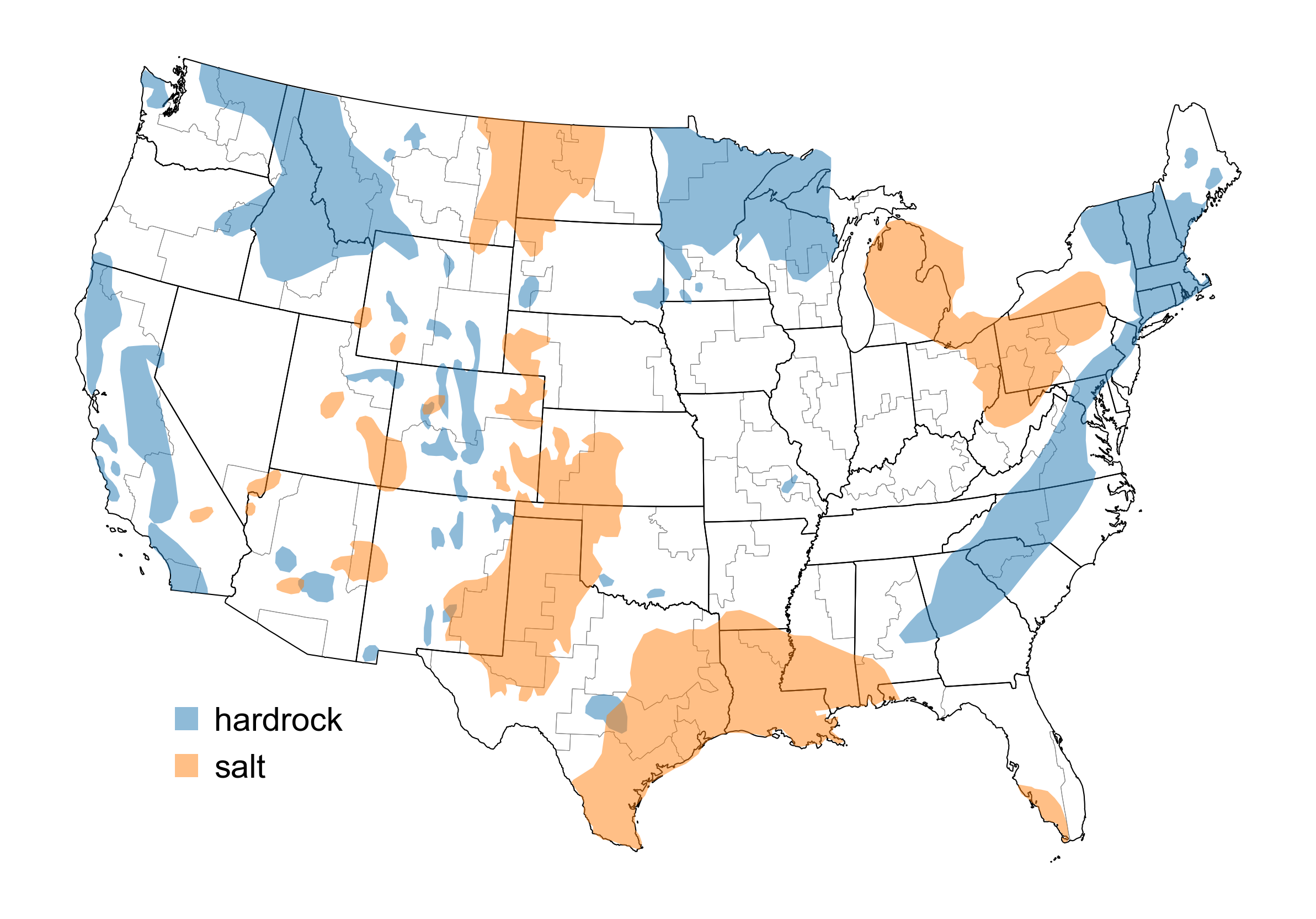
Fig. 35 Assumed availability of geological hydrogen storage reservoirs. Data are from [Lord et al., 2014].
Costs of hydrogen storage are based on estimates from [Papadias and Ahluwalia, 2021]. For geological storage, ReEDS assumes $/kg based on the economies of scale from constructing two to three caverns. To reduce model complexity, ReEDS assumes each zone can build only the cheapest storage option it has available. At least 1% of the region’s land area must overlap with the storage availability estimates from Fig. 35 for that storage type to be an option in that region. ReEDS requires any hydrogen storage be sized to hold at least 24 hours’ worth of hydrogen to run the H2-CTs in a given region. This minimum duration helps ensure the representative year has the storage needed to serve stress periods outside of the representative year.
ReEDS also allows the modeling of interzonal hydrogen transport. Transport requires the construction of hydrogen pipelines, and the model assumes cost estimates based on the H2 SERA model. Modeling hydrogen transport in ReEDS is an experimental feature and, because this feature adds significant runtime, the model includes the option to model zonal balancing with transport disabled or a fixed $/kg hydrogen transport cost.
Direct Air Capture
The model can also procure negative emissions by removing and storing CO2 from the atmosphere using direct air capture. DAC in the ReEDS model is represented as a sorbent design that uses only electricity as an input, with an energy consumption of 3.72 MWh per tonne of CO2 removed. Overnight capital costs are assumed to be $1,932 per tonne-year capture capacity, with annual FOM costs of 4.6% of the capital costs and nonfuel VOM costs of $21 per tonne.
CO2 Transport and Storage
ReEDS has the option to use a detailed CO2 network representation that, when turned on, requires all CO2 captured at CCS facilities (generation-based CCS, steam methane reforming with CCS, and DAC) to be transported via liquid CO2 pipelines and sequestered in underground saline aquifers. “Trunk” pipelines can be built between zonal transmission endpoints, and “spur” pipelines can be built from zonal transmission endpoints to the edge of any nearby (<200 mi) aquifer. These pipelines can be assigned different capital and FOM costs, and the several hundred saline aquifers identified by the National Energy Technology Laboratory have $/tonne breakeven costs that represent the cost of sequestering CO2 in the aquifer (i.e., permitting, injection facilities, monitoring, and a 100-year trust fund for maintenance).
The network representation includes only saline aquifers with a reservoir cost of <$20/tonne at a 90% capacity factor. The explicit representation is turned off by default.
Capital Stock
Initial capital stock, prescribed builds, and restrictions
Existing electricity generation capacity is taken from the EIA NEMS unit database [EIA, 2025] and updated using the March 2025 EIA 860M (Fig. 36). Units are mapped to ReEDS technologies based on a combination of fuel source and prime mover of the generation technology. Units of the same technology type within a region can be aggregated or represented individually.[17] If they are aggregated, the aggregation is done by clustering the units based on heat rates.
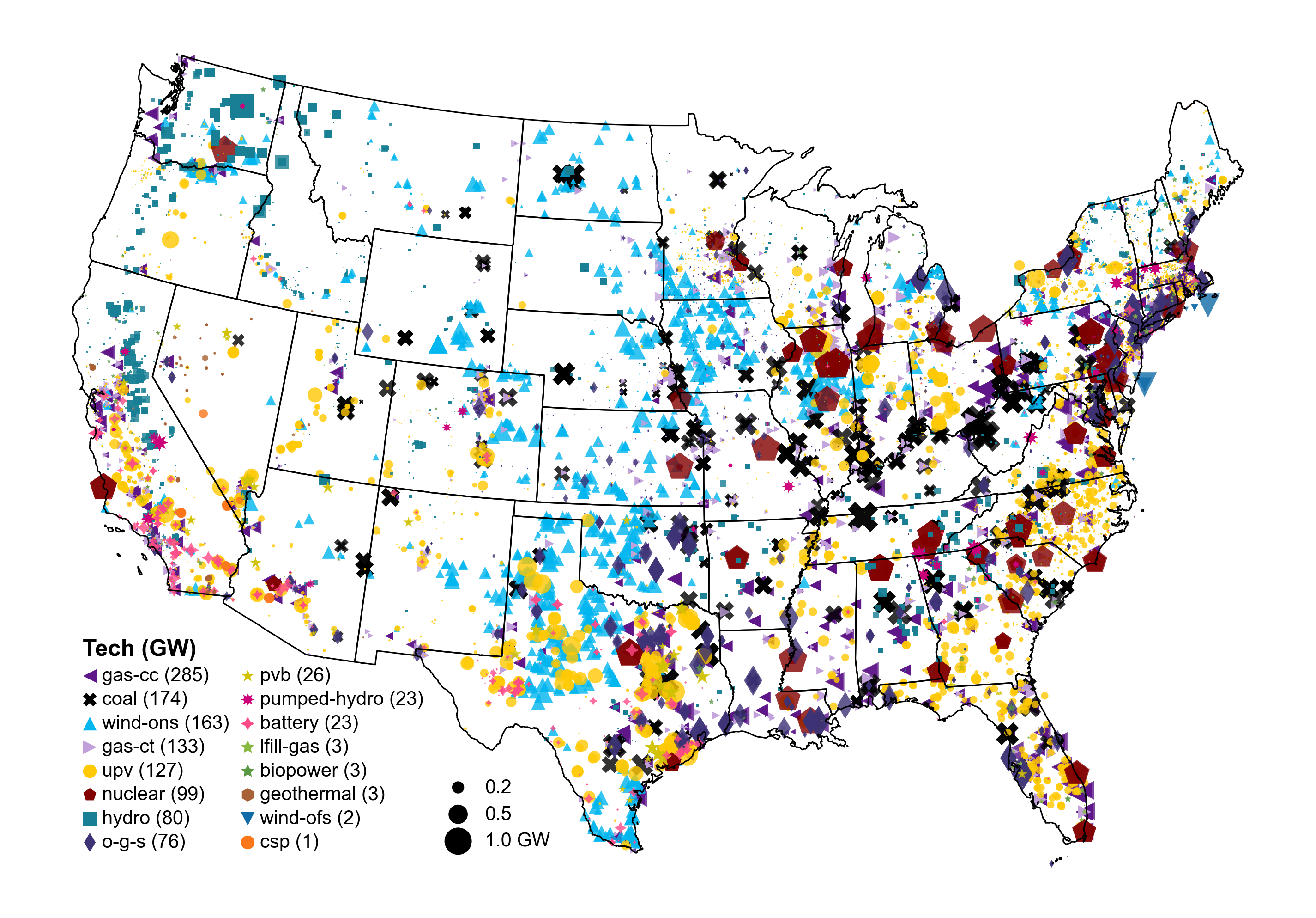
Fig. 36 Existing generation and storage units in 2025, taken from the EIA NEMS database [EIA, 2025].
The binning structure is designed flexibly so users can choose the appropriate levels of model fidelity and computational speed for each application. Historical units are binned using a k-means clustering algorithm for each zone and technology category (e.g., coal with or without SO2 scrubbers; natural gas combined cycle) combination. The user specifies a maximum number of bins and a minimum deviation across unit heat rates. Any two plants are eligible to form separate bins if the difference between their heat rates is greater than the minimum deviation parameter. The number of bins formed is then equal to the smaller of the maximum bin number parameter and the number of units after applying the minimum deviation criteria. For each bin, the assigned heat rate is equal to the capacity-weighted average of the heat rates for the units inside the bin.
Hydropower has additional subcategories to differentiate dispatchability as discussed in Hydropower.
Any plants that are listed as being under construction become prescribed builds.
In other words, ReEDS builds any under-construction units, with the units coming online in the anticipated online year listed in the database.
ReEDS also has the option to require nuclear demonstration plants to come online according to their announced dates.
That option is controlled by GSw_NuclearDemo, with the demonstration plant specifications and additional details in inputs/capacity_exogenous/demonstration_plants.csv.
This option is turned off by default.
Retirements
Renewable energy generator and battery retirements are (by default)[18] based on assumed lifetimes. Once a generator has reached its lifetime, it is retired. Renewable energy and battery lifetime assumptions are shown in Table 8. When renewable energy capacity is retired, the resource associated with that capacity is made available, and ReEDS can choose to rebuild a renewable energy generator using the newly available resource without the need to rebuild the grid interconnection infrastructure. A consequence of this assumption is retired renewable capacity can be replaced without incurring interconnection costs and, with all other considerations being equal, repowered or rebuilt renewable capacity has lower costs than new “greenfield” capacity of the same type.[19] One exception to this procedure is hydropower, which—because of assumed nonpower requirements—is never retired unless an announced hydropower capacity retirement is listed in the unit database.
Technology |
Lifetime (Years) |
Source |
|---|---|---|
Land-based Wind |
30 |
LBNL Survey [Wiser and Bolinger, 2019] |
Offshore Wind |
30 |
LBNL Survey [Wiser and Bolinger, 2019] |
Solar Photovoltaic |
30 |
SunShot Vision [DOE, 2012] |
Concentrating Solar Power |
30 |
SunShot Vision [DOE, 2012] |
Geothermal |
30 |
Renewable Electricity Futures Study, Vol. 1 [Mai et al., 2012] |
Hydropower |
100 |
Hydropower: Setting a Course for Our Energy Future [NREL, 2004] |
Battery |
15 |
Cole and Karmakar 2023 |
Hydrogen Electrolyzer |
20 |
|
Hydrogen Steam Methane Reforming and CCS |
25 |
|
Hydrogen Combined Cycle |
55 |
|
Hydrogen Combustion Turbine |
55 |
|
Biopower |
45 |
|
Gas Combustion Turbine |
55 |
|
Gas Combined Cycle and CCS |
55 |
|
Coal, all technologies, including cofired |
70 |
|
Oil-Gas-Steam |
55 |
|
Nuclear |
80 |
|
Nuclear SMR |
80 |
|
Compressed Air Energy Storage |
100 |
Retirement of existing fossil and nuclear capacity in ReEDS is primarily a function of announced retirement dates and technology-specific estimated lifetimes, taken from the AEO 2025 NEMS plant database and EIA 860M. Retirement dates of coal plants are further checked and updated in case the EIA 860M does not capture the latest retirement dates. Retirement dates for several nuclear plants, which are not current in NEMS and EIA 860M, are manually updated (Diablo nuclear power plants in California and Palisades nuclear power plant in Michigan). Both existing and economically built generators have the lifetimes shown in Table 8. These lifetimes are used as necessary when the solution period extends beyond 2050.
In addition to age-based retirements, ReEDS includes the option to endogenously retire technologies (this option is turned on by default). When doing endogenous retirements, ReEDS is trading off the value provided to the system by the plant versus the costs incurred by keeping the plant online. If the value is not sufficient to recover the costs, ReEDS will choose to retire the plant. ReEDS includes a “retirement friction” parameter that allows a plant to stay online as long as it is recovering at least a portion of its fixed operating costs. For example, if this retirement friction parameter is set to 0.5, a plant will retire only if it does not recover at least half of its fixed costs. In addition, ReEDS includes a minimum retirement age for existing fossil and nuclear plants of 20 years, meaning a fossil or nuclear plant is not allowed to be endogenously retired until it is at least 20 years old.
Growth constraints
The ReEDS model can represent either absolute growth constraints (e.g., wind builds cannot exceed 100 GW per year) or relative growth constraints (e.g., wind capacity cannot grow by more than 50% per year). The growth constraints are designed to target a broader technology group as opposed to the individual classes of wind, PV, and CSP; as an example, the growth constraint would restrict the builds of all wind technologies and classes and not just a specific class. The default values for the absolute growth constraints are the highest year-over-year changes of each technology type’s capacity from 2010 to 2020. For CSP, the default absolute growth limit is assigned the same as PV, because it has not seen the capacity buildout as PV or wind has as of 2020. The relative growth limits are applied on a state level and are based on historical compounded annual growth rate estimates observed for solar PV from 2012 to 2022. The penalties are assessed in ReEDS based on the maximum previous growth observed in the model. For example, if a state experienced 1,000 MW of new capacity in 2024 and 500 MW of new capacity in 2025, the growth penalty would be applied using the 1,000-MW value even though it is older.
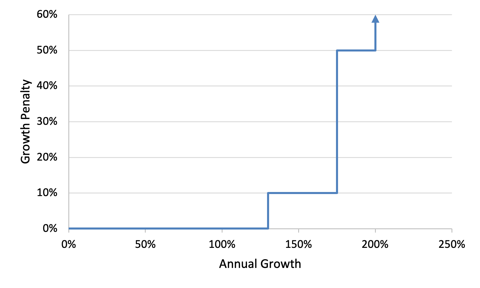
Fig. 37 Annual growth penalties applied on a state level in ReEDS when the relative growth penalties are enabled.
ReEDS also includes minimum growth sizes, specified by technology type. These minimum growth sizes are shown in Table 9 and are generally based on representative plant sizes.
Technology group |
Minimum growth size before a penalty is incurred (MW) |
|---|---|
Battery |
100 |
Biomass |
50 |
CSP |
100 |
Natural Gas |
300 |
Hydrogen |
100 |
Hydropower |
100 |
Nuclear |
600 |
Pumped Storage Hydropower |
600 |
Solar PV |
100 |
Storage |
100 |
Wind-Offshore |
600 |
Wind-Onshore |
100 |
Interconnection queues
To incentivize near-term capacity deployments to be more aligned with the current grid interconnection capacity queues as of the end of 2024 [Rand et al., 2025],
ReEDS includes a constraint that limits capacity deployment and refurbishment by technology and ReEDS region,
starting in user-defined interconnection_start year (which can be specified in inputs/scalars.csv) and ending in 2030.
The 2026 limits are based on plants with a signed interconnection agreement, and the 2030 limits are based on the total amount of capacity seeking interconnection (see inputs/capacity_exogenous/interconnection_queues.csv).
Values between years are interpolated based on the 2026 and 2030 points.
The limits are applied regionally by technology.
To avoid infeasibility, the constraint allows a technology to be built over the capacity limits with a penalty of $10,000/kW.
Regional Parameter Variations and Adjustments
For most generation technologies, regional cost multipliers are applied to reflect variations in installation costs across the United States (see Fig. 38). These regional multipliers are applied to the base overnight capital cost presented in earlier sections. The regional multipliers are technology-specific and are derived primarily from the EIA/Leidos Engineering report [EIA, 2016] that is the source of capital cost assumptions for the NEMS model. Although the regional costs presented in the EIA/Leidos Engineering report are based on particular cities, the regional multipliers for ReEDS are calculated by interpolating between these cities and using the average value over the ReEDS regions for each technology. For technologies such as CSP that are not included in the newer report, we rely on the older EIA/Science Applications International Corporation report [EIA, 2013].
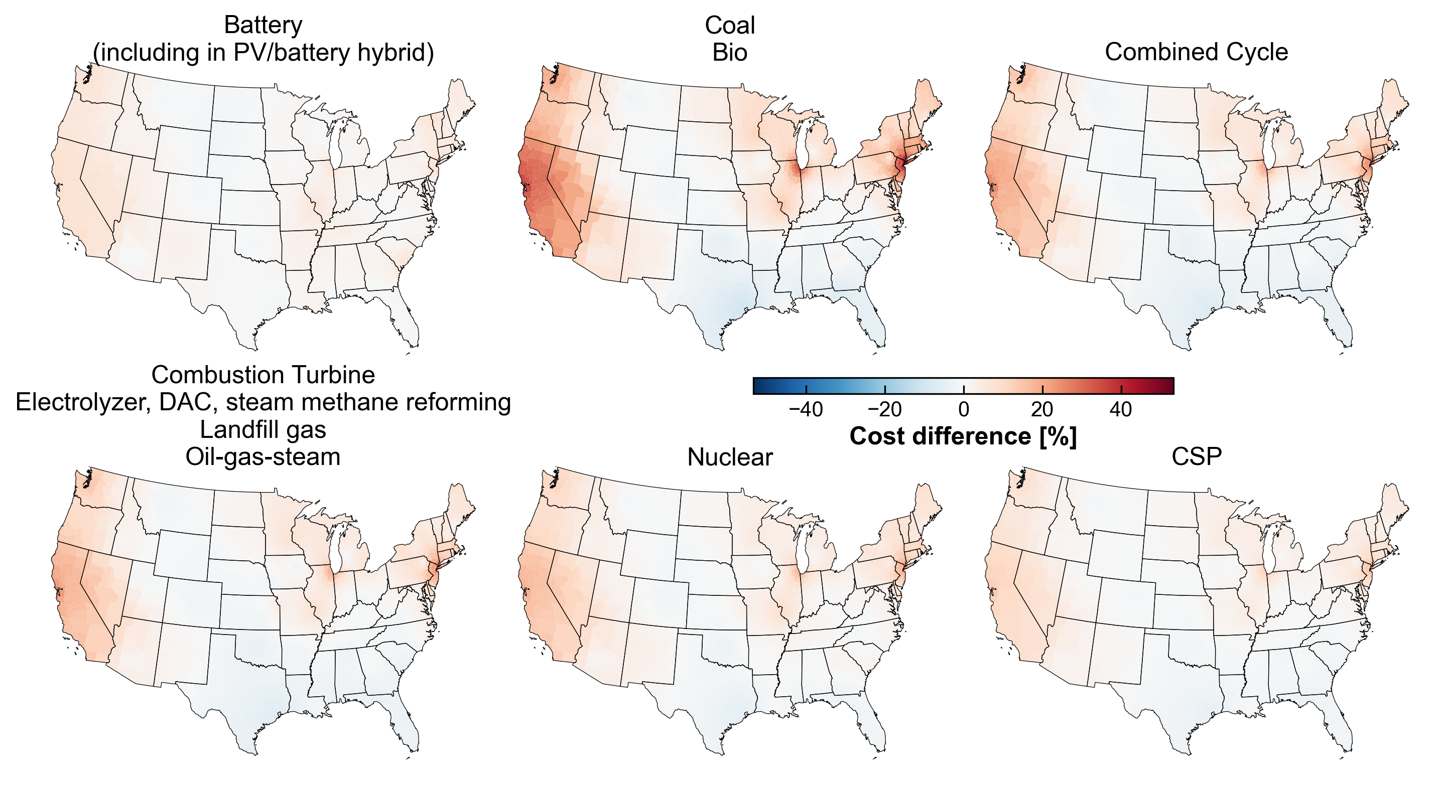
Fig. 38 Maps of regional capital cost multipliers for the various technology types.
Regional capital cost multipliers for the above technologies are available at zonal resolution. The capital cost multipliers for PV, land-based wind, and offshore wind are incorporated upstream in the supply curves produced by reV; therefore, the multipliers used in ReEDS for these technologies are set to 1.0 to avoid double counting.
Outage Rates
Forced outages for combined cycle, combustion turbine, nuclear (conventional and SMR), steam (coal), nuclear, hydro and pumped hydro, and diesel generators are modeled using temperature-dependent forced outage rates from [Murphy et al., 2019]. Some regions experience air temperatures outside the -15–35°C range reported in [Murphy et al., 2019]; outage rates outside this temperature range are linearly extrapolated up to a maximum of 40%, where 40% is the ELCC derate applied to gas combustion turbines in [PJM, 2025]. Fig. 39 shows the resulting forced outage rates as a function of temperature. Forced outage rates for other technologies are taken from the NERC Generating Availability Data System (GADS) database [NERC, 2023] for 2014–2018 and are applied as time-invariant average values.
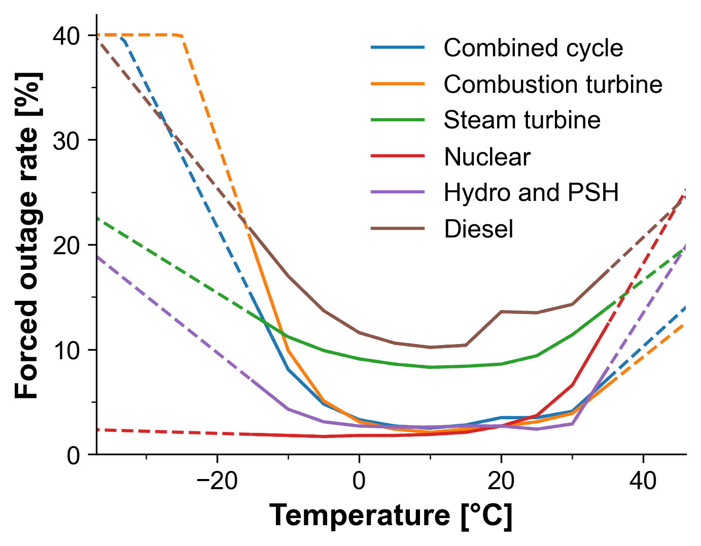
Fig. 39 Forced outage rates as a function of temperature. Solid lines indicate the portion of the data taken from [Murphy et al., 2019]; dashed lines indicate extrapolated data.
Hourly surface air temperatures for all weather years are taken from the NSRDB [National Renewable Energy Laboratory, 2024]. Temperatures are averaged over each model zone, and the hourly average temperatures are converted to hourly forced outage rates using the relationships shown in Fig. 39. Fig. 40 shows illustrative monthly average forced outage rates for gas combustion turbines and nuclear.
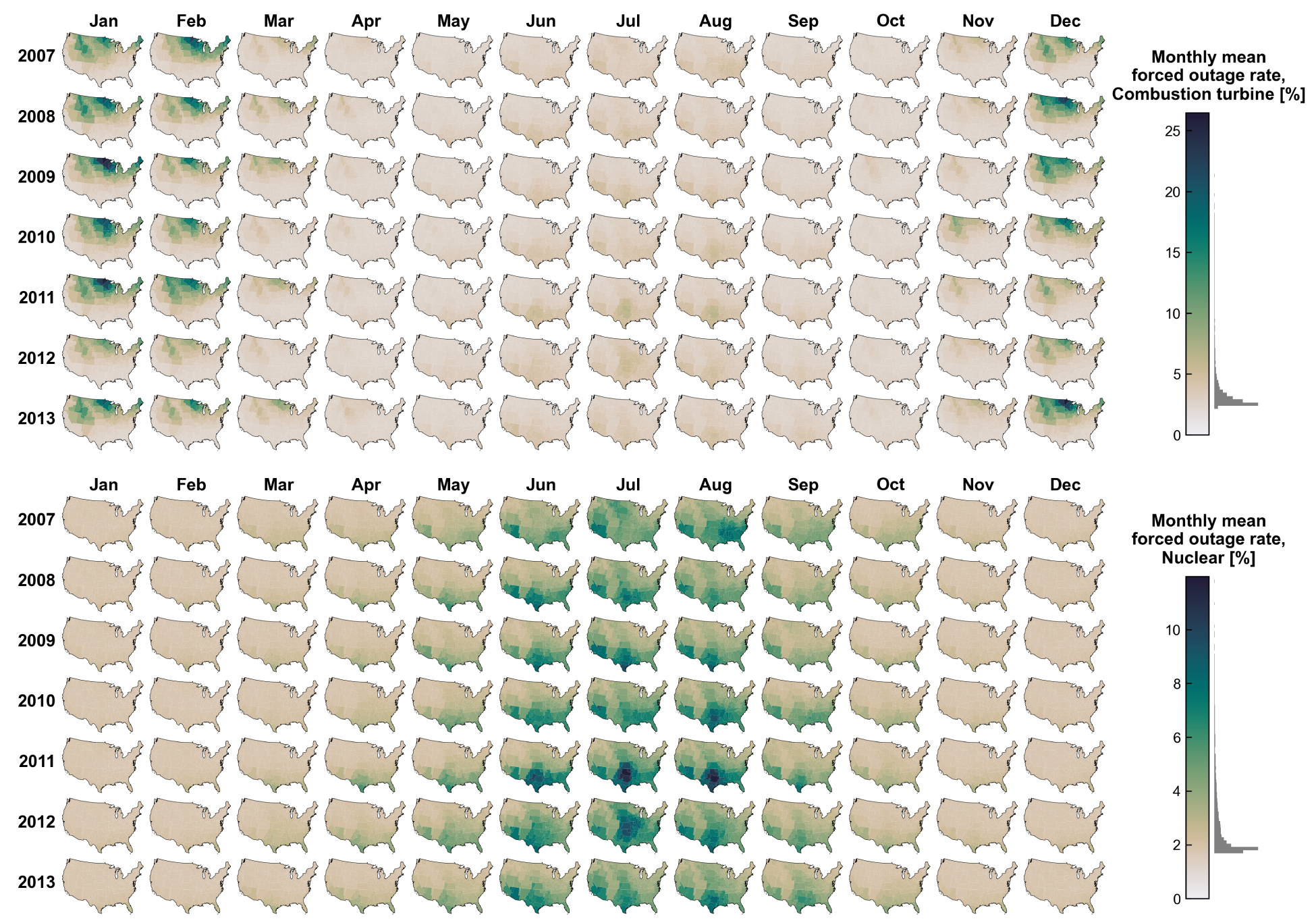
Fig. 40 Example forced outage rates for gas combustion turbines (top) and nuclear (bottom). Note the difference in color scales.
Scheduled (planned and maintenance) outage rates are derived from the NERC GADS database [NERC, 2023]. Scheduled outage rates for combined cycle, combustion turbine, nuclear, steam (coal), and hydro technologies are measured and applied at monthly resolution using GADS data from 2013 to 2023 [Murphy, 2025]. Scheduled outage rates for other technologies are measured as time-independent average values using GADS data from 2014 to 2018; scheduled outages for these technologies are applied only during spring and fall, with the outage rates during those months scaled to reproduce the measured time-independent averages. Fig. 41 shows scheduled outage rates for the technologies used by default.
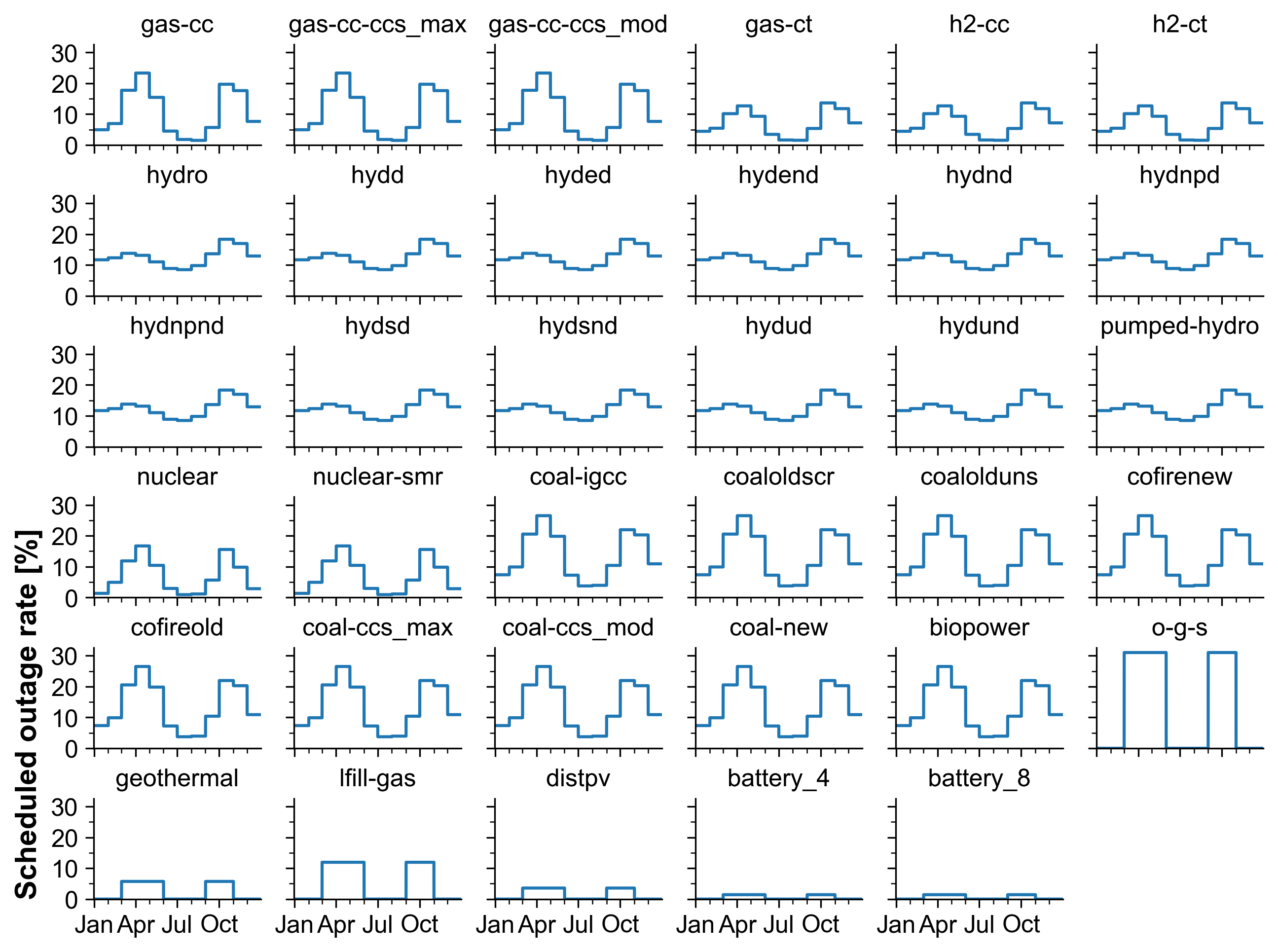
Fig. 41 Scheduled outage rates for the default collection of technologies.
Outage rates for wind power are handled upstream in the reV model and included in the hourly capacity factor profiles, as described by [Lopez et al., 2025]. In addition to static losses of 11% (including the effects of forced and scheduled outages) and endogenously modeled hourly wake losses (ranging from 0.05% to 25%), two types of weather-driven shutoffs are considered, both of which are assumed to reduce site-level wind generation to zero in affected hours: extreme cold shutoffs, applied when air temperature at hub height reaches ≤-20°C, and shutoffs for potential icing events, applied when air temperature reaches ≤0°C and relative humidity reaches ≥95%. Fig. 42 shows an example week illustrating these shutoffs for a site near Fargo, North Dakota.
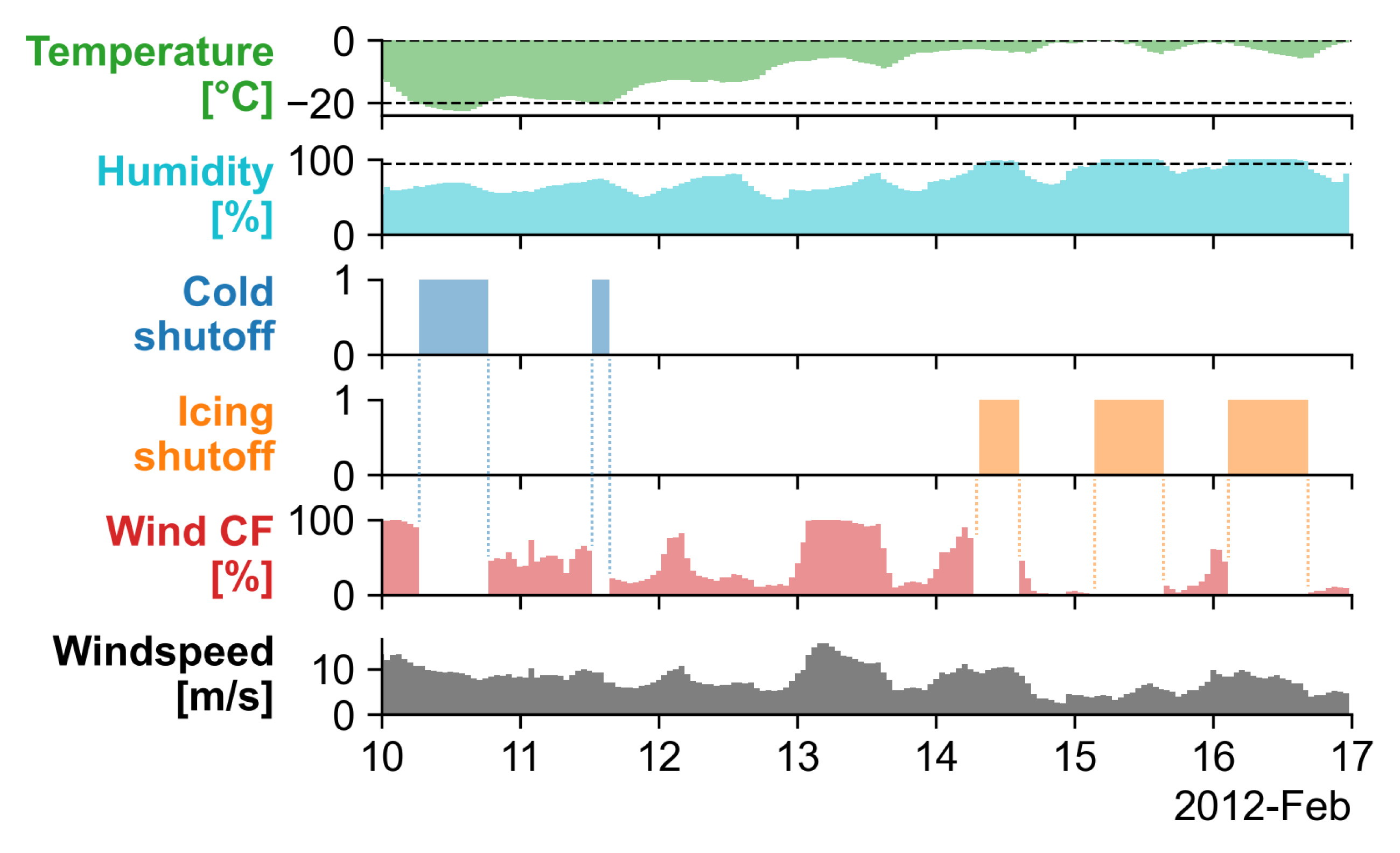
Fig. 42 Air temperature, relative humidity, cold/icing shutoff indicators, modeled wind capacity factor, and wind speed for an example week at a site near Fargo, North Dakota.
Fuel Prices
Natural gas, coal, and uranium prices in ReEDS are based on the AEO2025. Coal prices are taken from the Reference scenario, with any missing values from the Reference scenario forward-filled using prior years. Coal prices are provided for each of the nine EIA census divisions. Default natural gas prices and demand levels are from the AEO2025 Reference scenarios. Low and high natural gas price alternatives are taken from the High and Low Oil and Gas Resource and Technology scenarios, respectively. ReEDS includes only a single national uranium price trajectory based on the AEO2025 Reference scenario. Base fuel price trajectories are shown in Fig. 43 for the AEO2025 [EIA, 2025]. Biomass fuel prices are represented using supply curves as described in the Biopower section.
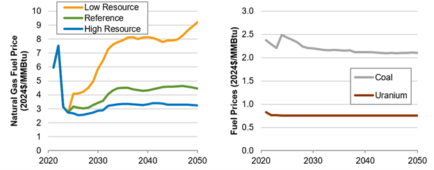
Fig. 43 Input fuel price assumptions.
Natural gas fuel prices are adjusted by the model as explained below.
Coal and uranium are assumed to be perfectly inelastic; the price is predetermined and insensitive to the ReEDS demand for the fuel. With natural gas, however, the price and demand are linked. Actual natural gas prices in ReEDS are based on the AEO scenario prices but are not exactly the same; instead, they are price-responsive to ReEDS natural gas demand. In each year, each census division is characterized by a price-demand “setpoint” taken from the AEO Reference scenario but also by two elasticity coefficients: regional (\(\beta_r\)) and national (\(\beta_{\text{nat}}\)) elasticity coefficients for the rate of regional price change with respect to 1) the change in the regional gas demand from its setpoint and 2) the overall change in the national gas demand from the national price-demand setpoint, respectively. The set of regional and national elasticity coefficients is developed through a linear regression analysis across an ensemble of AEO scenarios[20] to estimate changes in fuel prices driven solely by electric sector natural gas demand (as described in [Logan et al., 2013] and [Cole et al., 2016], although the coefficients have since been updated for the latest AEO data). Although there is no explicit representation of natural gas demand beyond the electricity sector, the regional supply curves reflect natural gas resource, infrastructure, and nonelectric sector demand assumptions embedded within the AEO modeling. For details, see the Natural Gas Supply Curves section of the appendix.
ReEDS includes options for other types of fuel supply curve representations. Supply curves can be national-only, census-division-only, or static. With the national-only supply curve, there are census division multipliers to adjust prices across the census divisions. In the static case, fuel prices are not responsive to demand.
Transmission assumptions
The switch GSw_GasCurve controls the choice of natural gas supply curve.
0 = census-division-only, 1 = national + census division, 2 = static, 3 = national-only
The natural gas fuel prices also include a seasonal price adjustor, making winter prices higher than the natural gas prices seen during the other seasons of the year. For details, see the Seasonal Natural Gas Price Adjustments section of the appendix.
Electricity Demand
End-use electricity demand is an exogenous input to ReEDS represented by hourly profiles. The available load profile options fall into three categories: 1) load projections from Evolved Energy Research, 2) load projections developed as part of the Electrification Futures Study and 3) historic load multiplied by annual load growth factors from AEO. When applicable, ReEDS will modify the exogenously specified profiles by applying a load shape adjustment method that incorporates analysis from other modeling tools or by adding load from endogenously built electricity-consuming technologies.
ReEDS includes interzonal transmission system losses in the optimization but does not represent distribution losses. To account for this, the end-use load must be scaled up by a distribution loss factor to convert it to busbar load. A distribution loss factor of 5%, which is estimated based on a combination of EIA and ReEDS numbers, is used for this conversion. Note that distribution losses do not apply to rooftop PV generation because this generation is assumed to be used locally within the distribution network. ReEDS is required to generate sufficient power to meet busbar load (allowing for transmission of power but accounting for losses) in each hour and zone.[21]
Evolved Energy Research Load Profiles
The load profiles from Evolved Energy Research (EER) are the newest load profile addition to the model. EER builds hourly, state-level load profiles for each end-use sector, disaggregates them to the ReEDS zone level, and then aggregates them across sectors to produce the total end-use load profiles used in ReEDS. The profiles feature 15 weather years of data (2007–2013 and 2016–2023), allowing us to compute resource adequacy based on a wide variety of weather conditions. There are three sets of EER profiles, each reflecting different electrification assumptions: EER_Baseline_AEO2023, EER_IRAlow, and EER_100by2050. EER_Baseline_AEO2023 reflects business-as-usual electrification based on load estimates from AEO2023. EER_IRAlow reflects the impacts of the Inflation Reduction Act (IRA), which features many tax credits and subsidies for electric end-use technologies such as electric vehicles and heat pumps. Specifically, EER_IRAlow “reflects relatively conservative assumptions about the impact of demand-side provisions in the Inflation Reduction Act (relative, compared to other scenarios developed by EER)” [Gagnon et al., 2024]. EER_100by2050 reflects the electrification required to reach 100% economywide decarbonization by 2050. ReEDS defaults to EER_IRAlow. Compound annual growth rates (CAGRs) and 2050 CONUS-wide annual demand for each set of profiles is shown in Table 10.
CAGR (2025 through 2050) |
2050 CONUS-wide Electric Load (TWh/year) |
|
|---|---|---|
EER_Baseline_AEO2023 |
1.2% |
5,504 |
EER_IRAlow (default) |
1.8% |
6,402 |
EER_100by2050 |
2.7% |
7,975 |
Electrification Futures Study Load Profiles
ReEDS also contains detailed electrification load profiles developed as part of the Electrification Futures Study using EnergyPATHWAYS [Sun et al., 2020]. The profiles use one weather year of data (2012). Because there is only a single weather year, the model duplicates these profiles to match the number of weather years specified by the user. Note that this results in loss of synchronicity between demand and other weather-based data when weather years beyond 2012 are selected. There are five sets of profiles, each reflecting different electrification assumptions: EPREFERENCE, EPMEDIUM, EPMEDIUMStretch2040, EPMEDIUMStretch2046, and EPHIGH. EPREFERENCE serves as a baseline of comparison to the other scenarios, featuring the least incremental change in electrification through 2050. EPMEDIUM features widespread electrification among the “low-hanging fruit” opportunities in electric vehicles, heat pumps, and select industrial applications. EPMEDIUMStretch2040 and EPMEDIUMStretch2046 are modified versions of EPMEDIUM that lower the aggressiveness of its electrification assumptions by “stretching” its load growth through 2040 and 2046 respectively out to 2050 such that total 2040 and 2046 load from EPMEDIUM are equivalent to 2050 load from EPMEDIUMStretch2040 and EPMEDIUMStretch2046 respectively. EPHIGH features a combination of technology advancements, policy support, and consumer enthusiasm that enables transformational change in electrification. The 2050 CONUS-wide annual demand and overall peak CONUS-wide demand for each set of profiles is shown in Table 11.
2050 CONUS-wide Electric Load (TWh) |
Peak CONUS-wide Electric Load (GW) |
|
|---|---|---|
EPREFERENCE |
4,788 |
852 |
EPMEDIUMStretch2040 |
5,062 |
963 |
EPMEDIUMStretch2046 |
5,499 |
1,049 |
EPMEDIUM |
5,799 |
1,104 |
EPHIGH |
6,699 |
1,279 |
Historical Load Data + AEO Growth Factor Profiles
Load can also be modeled in ReEDS with historical hourly profiles multiplied by load growth factors from AEO. The historical profiles feature 15 weather years of data (2007–2013 and 2016–2023), with the pre-2014 and post-2015 profiles created using distinct methodologies, which are described below.
For 2007–2013, historic hourly load data are collected for each year at the utility region level from FERC Form 714 and the RTO/independent system operator (ISO) region level from RTO/ISO websites. Interannual load growth is removed from these profiles using regional load growth factors. Specifically, the profiles for years outside of 2012 are “ungrown” such that their annual regional totals approximately match those of the 2012 profiles. The ungrown profiles are then converted to the ReEDS zone level. This is done by first determining the buses that exist in each region and allocating each region’s load to its buses using bus-level load participation factors from Energy Visuals. The buses are then mapped to ReEDS zones, based strictly on bus location and ReEDS zone boundaries, and the bus-level load is re-aggregated to the ReEDS zone level. Using retail energy load data from EIA’s Electricity Data Browser [EIA, 2015], the zonal load profiles for each year are then scaled such that the annual total load of the zones comprising a given state roughly matches that state’s total 2010 retail sales of electricity.
For 2016–2023, historic hourly load data are collected for each year at the NERC balancing authority region and subregion level from EIA Form 930 and RTO/ISO websites. The profiles are then downscaled to the county level and re-aggregated to the ReEDS zone level.
The historic load profiles are combined to create a full 15-year dataset, and a method developed by Evolved Energy Research is applied to the dataset to remove interannual load growth. Specifically, for each zone, a linear regression model is fitted to the 2016–2023 subset of the zone’s load profile, with time as the predictor variable and load as the response variable, and then the regression model is used to generate a predicted load value at each hour, the full set of which represents the trend of the profile. The load profile is then “detrended” by subtracting the trend from it (i.e., subtracting the predicted load value at each hour from the actual load value at that hour) and then rescaled to roughly match 2023 load by adding to each hourly load value the last value of the trend (i.e., the predicted load value associated with the final hour of 2023). For each zone and weather year from 2007 to 2013, that year’s subset of the zone’s load profile is scaled such that total annual load matches the average annual load of the detrended 2016–2023 data.
State-level load growth factors for 2010–2050 are obtained from AEO for each of their electricity consumption scenarios - low, reference, and high. For each zone and model year in ReEDS, the zone’s load profile is scaled according to the growth factor of the zone’s state for that year, with the load profile’s shape remaining constant throughout the study period.
Load Adjustment Method for End-Use Profiles
ReEDS includes a methodology to incorporate changes to hourly electric load shapes derived from analysis of other modeling tools. Regional hourly load changes are paired with a defined regional adoption trajectory for this load change by year. Combining these two factors allows ReEDS to change to load profiles specific to region, year, and hour. A further unique capability of this method is that an arbitrary number of load changes and adoption trajectories can be provided, allowing sophisticated changes to load shapes with a small number of provided parameters.

Fig. 44 ReEDS load adjustment method.
This methodology allows ReEDS load profiles to be adjusted quickly within an analysis scenario. This methodology is based on methods developed to incorporate changes to electric power demand associated with geothermal heat pumps; example hourly change profiles and adoption scenarios derived from that analysis are available.
Endogenous Load
ReEDS models a few electricity-consuming technologies that, when built and operated in the model, can endogenously increase the load profile in addition to the exogenously specified profiles discussed above.
Those electricity-consuming technologies are electrolyzers, steam methane reforming with or without CCS, and DAC.
These technologies are assumed to consume electricity at the wholesale electricity price.
ReEDS users can alter this assumption with the GSw_RetailAdder switch, which adds a 2004$/MWh cost adder to electricity consumed by these technologies.
Demand Response
Demand response (DR) is turned off by default in ReEDS, but the user has the option to enable DR via load shedding. The demonstration data used to characterize the amount of load shedding avaiable were obtained from a workflow which includes ResStock, DR-Path, and dsgrid. The data reflect the technical potential for residential load shedding in 11 states (AZ, CA, CO, FL, GA, MN, MT, NM, NY, TX, WA) and were developed using the 2018 weather year. Through this implementation the demand response is effectively added as a new supply curve-based resource; however, the DR shed potential is only available during stress periods. If ReEDS chooses to dispatch DR shed, the “generation” from the resource is subtracted from the load considered in the resource adeqaucy calculations. The capital costs for the residential resource are derived from the installation cost for the DR-enabling technology (program implementation or procurement costs are not included). In addition to only allowing the shed resource to be dispatched during stress periods, a max daily capacity factor is defined. For the residential heating and cooling resources the max daily capacity factor is set to 4 hours per day.
Transmission
ReEDS considers two categories of transmission: “local interconnection” of generation capacity within the model zones and “interzonal” or “long-distance” transmission between the model zones. These two categories of transmission share underlying cost data but are represented differently within the model. Transmission costs are described first, followed by the separate representations of “local interconnection” and “interzonal” (or “long-distance”) transmission within ReEDS.
Transmission Costs
Estimated costs for transmission lines are generated by defining a high-geographic-resolution cost surface, then using a least-cost-path algorithm to identify a representative transmission line path between two points [Lopez et al., 2025]. The final $/MW cost for a particular route is then given by the integrated $/MW-mile values for the cost surface points traversed by the least-cost route.
Base voltage-dependent $/MW-mile transmission costs are taken from four sources: Southern California Edison for California Independent System Operator (CAISO) and the Northeast, Western Electricity Coordinating Council/Transmission Expansion Planning Policy Committee (WECC/TEPPC) for non-CAISO areas in the Western Interconnection, Midcontinent Independent System Operator (MISO) for the Midwest, and a representative utility for the Southeast. These base transmission costs are shown on the left side of Fig. 45. Cost multipliers based on terrain type (hilly, with land slope between 2% and 8%, and mountainous, with ≥8% land slope) and land class (pasture/farmland, wetland, suburban, urban, and forest) are taken from the same four sources. A separate 90-m-resolution CONUS dataset of terrain and land classes is then combined with the base transmission costs, terrain multipliers, and land class multipliers to generate the cost surface used in the least-cost-path routing algorithm.

Fig. 45 Overview of transmission cost input data used in reV model calculations, used to generate ReEDS model inputs.
Transmission of all types (local and interzonal) incurs FOM costs, which are approximated as 1.5% of the upfront capital cost per year [E. Weidner et al., 2014].
Local Generator Interconnection
There are three components of local generator interconnection represented in ReEDS: geographically resolved spur lines and substation upgrades, geographically resolved reinforcement of the existing transmission network, and a geographically independent cost adder for all technologies. The methods for calculating geographically resolved spur line and network reinforcement costs are described in detail by [Lopez et al., 2025] and briefly outlined below.
Spur lines and substation upgrades
Spur lines represent short-distance transmission built to connect new wind and solar generation capacity to a “point of interconnection” on the existing transmission system. For a given wind/solar site (the ~50,000 reV supply curve points discussed above), existing substations and high-voltage transmission lines (taken from [Homeland Infrastructure Foundation Level Database (HIFLD), 2024]) within the same state are considered possible POIs. Least-cost paths are calculated to all candidate POIs (assuming 138 kV for all spur lines), and the POI with the lowest resulting path-dependent spur line cost is taken as the POI for that wind/solar site. Substation POIs incur a substation upgrade cost of $15/kW; transmission line POIs incur a new-substation cost of $35/kW.
Network reinforcement
Network reinforcement represents upgrades to the existing transmission network required to avoid congestion when moving power from the POI for a new generator to load centers. It is intended to represent the costs associated with interconnection queues, which represent a major bottleneck for the deployment of new wind and solar in the United States. [Gorman et al., 2025]. Network reinforcement costs are approximated by tracing a path along existing transmission lines from each wind/solar POI to each zone “center” within the same state; the zone center is usually taken as the largest population center in the model zone but is sometimes (for zones without large urban centers) assigned to a high-voltage substation within the zone.[22] A cost for each reinforcement route is calculated using the cost surface described in Transmission costs, with capital expenditure (CAPEX) costs multiplied by 50% to approximate the lower cost for reconductoring compared to greenfield transmission construction. The single lowest-cost route for each POI is then selected; the associated reinforcement cost [$/MW] and transmission distance [MW-miles] are incurred for every MW of new wind/solar capacity added at all reV sites associated with that POI. (This heuristic method of tracing a path from the POI to the largest load center in the zone is highly simplified and does not represent all the considerations involved in an actual interconnection study.)
Fig. 46 illustrates the concepts of spur lines and reinforcement lines, and Fig. 47 shows the resulting distribution of interconnection costs for land-based wind and utility-scale PV under the three siting regimes.
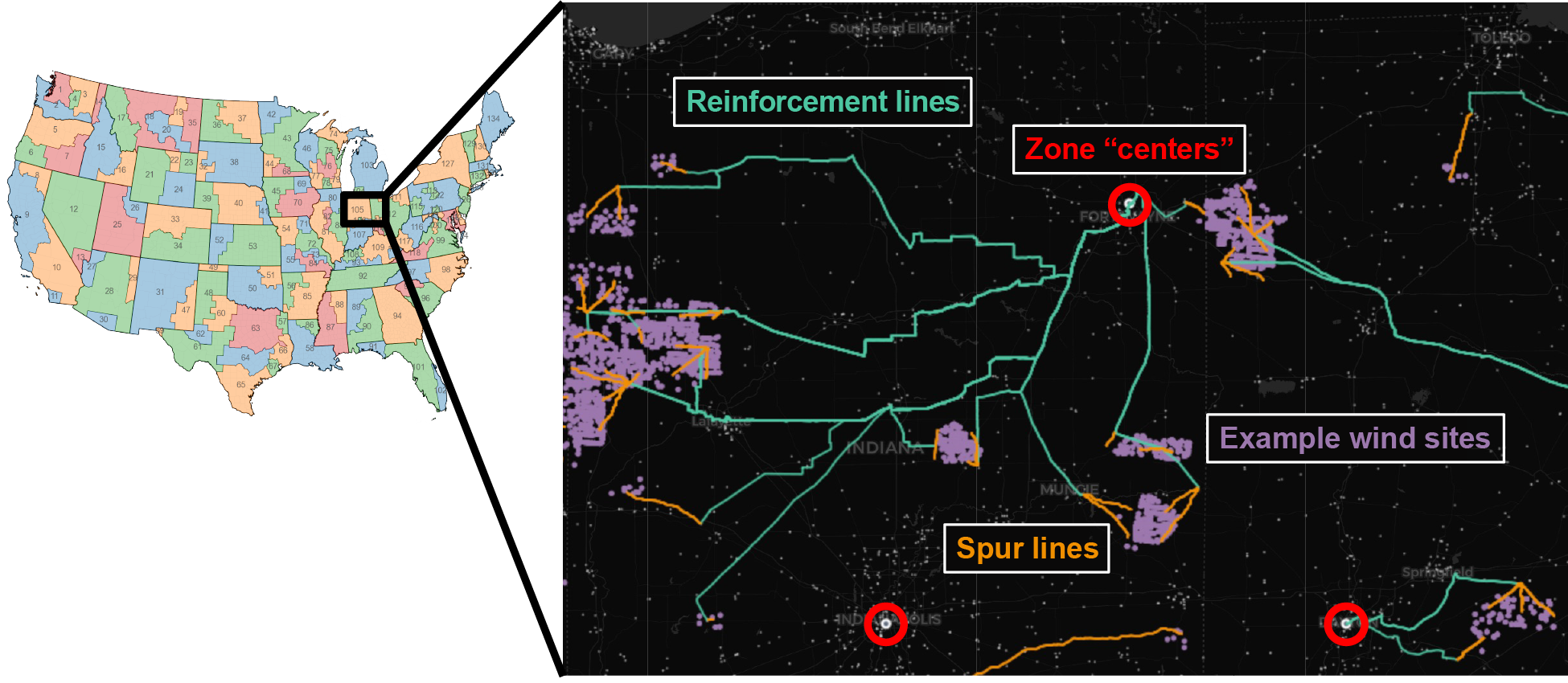
Fig. 46 Illustration of local generation interconnection components.
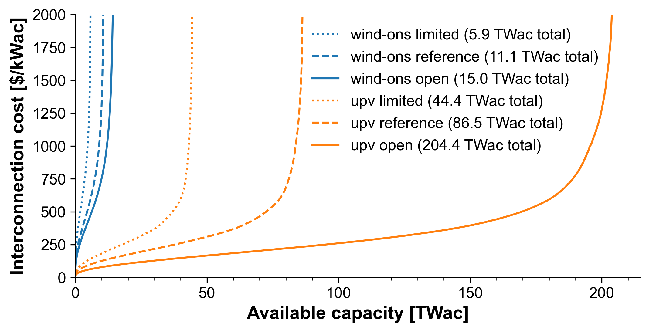
Fig. 47 Interconnection cost distribution for land-based wind (blue) and utility-scale PV (orange) under different siting assumptions.
Fig. 48 shows maps of the estimated spur line costs, reinforcement costs, total interconnection costs, and total supply curve costs (including land-cost adders) by reV site.
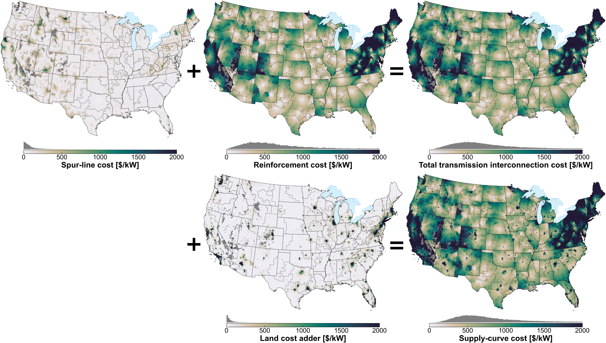
Fig. 48 Supply-curve costs by reV site. Data are for utility-scale PV with open-access siting but are similar for other technologies and siting access assumptions.
Spur lines and network reinforcement use the same financial multiplier as the generation technology they are associated with.
Intrazone transmission cost adder for net increases in generation capacity
In addition to the interconnection costs described above, a flat intrazone transmission cost adder of $100/kW is also applied to net increases in generation and AC/DC converter capacity within each model zone. This value is taken from historical interconnection costs for fossil gas capacity [Seel et al., 2023] and is taken to represent a “floor” for network upgrades that are required even if new capacity is added at the optimal location (assuming past additions of fossil capacity have been placed to minimize interconnection costs). The $100/kW adder is subtracted from the reinforcement cost applied to wind and solar to avoid double counting. Because new generation capacity is assumed to reuse the network infrastructure from retiring capacity, the intrazone transmission cost adder is applied only to net increases in generation capacity.
This generation-technology-neutral intrazone transmission cost adder uses a financial multiplier calculated using a 40-year capital recovery period.
Interzonal Transmission
Interzonal transmission flows in ReEDS are modeled using a simple energy balance and transport model (sometimes called a “pipe and bubble” or “pipe flow” approach) between model zones, with each zone treated as a “copper plate” (i.e., without monitoring flows or enforcing flow limits within zones). Within each zone, electricity generation and imports, minus interzonal demand and exports, must sum to zero; interzonal flows are constrained by the MW capacity of each interzonal interface (which can be expanded, as discussed below).
Four types of interzonal transmission are considered in ReEDS: alternating current (AC), representing the large majority of existing U.S. capacity; point-to-point high-voltage direct current (HVDC) with line commutated converters (LCC); meshed multiterminal HVDC with voltage source converters (VSC); and back-to-back (B2B) AC/DC/AC converters.
Existing AC interface capacities are calculated using a nodal DC power flow model, but within the ReEDS linear optimization, the balance of flows between interfaces is not constrained by optimal power flow.
The representation of existing interzonal transmission capacity is discussed first, followed by the representation of new interzonal transmission capacity additions.
Existing transmission capacity
AC
Interface transfer limits (ITL) are calculated as described by [Brown et al., 2023]. (The ITL is similar to the total transfer capability metric used elsewhere [Mohammed et al., 2019, NERC, 2024], but the ITL uses more flexible assumptions for load and generation.) In this calculation, the existing transmission system is approximated using the nodal network model developed for the North American Renewable Integration Study [Brinkman et al., 2021], which represents a 2017-era projection of a then-future 2024 network. For each interzonal interface (where an interface is defined as the collection of transmission lines that cross between a pair of model zones), a linear optimization is performed to determine the collection of transmission line flows and nodal injections and withdrawals that maximize the power flow across the interface, subject to constraints on individual line ratings, the relationship between nodal injections/withdrawals and line flows as governed by the power transfer distribution factor matrix, nodal load distributions as determined by fixed load participation factors, and a requirement that generation buses can only inject power to the network and load buses can only withdraw power from the network. Published WECC path limits are also applied as constraints on the combined line flow for the lines that comprise each path [Western Electricity Coordinating Council, 2022]. A separate, independent optimization is performed for each direction on each interface; in general, the ITL for power flow from Zone A to Zone B is not the same as the ITL for power flow from Zone B to Zone A.
As discussed in [Brown et al., 2023], because of the constraints imposed by Kirchhoff’s voltage law and nodal load participation factors, the ITL tends to be smaller than the sum of line ratings that cross an interface; that is, every transmission line between a pair of regions cannot in general be used at their rated capacities at the same time. The same effect is observed for larger interfaces; when modeled at nodal resolution, the maximum flow between SPP and MISO (for example) is smaller than the sum of the zonal ITLs for the zonal interfaces that span the larger SPP-MISO interface. For this reason, transmission flows are constrained at two levels within ReEDS, illustrated in Fig. 49: between the model zones (gray bars) and between the planning subregions (black bars).
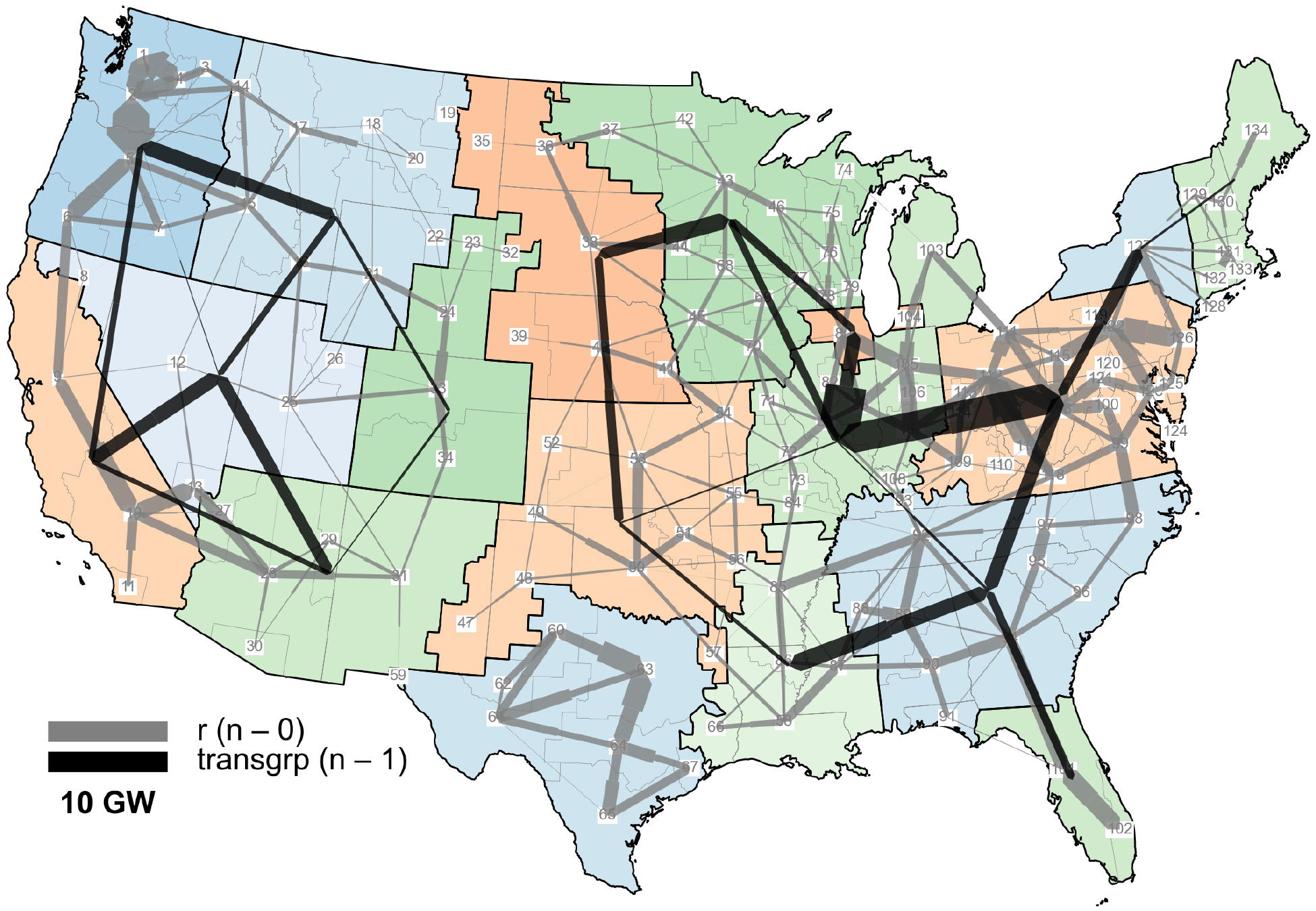
Fig. 49 Existing AC transmission capacity in ReEDS.
For the planning region ITLs, \(n - 1\) contingency considerations are approximated by dropping the interregional line that contributes the most capacity to the calculated ITL for each interregional interface and flow direction, then recalculating the ITL with that line removed. ITLs between model zones are calulcated under \(n - 0\) conditions—i.e., without accounting for contingency events. Because the ITLs are applied simultaneously for all interfaces during the ReEDS optimization, applying \(n - 1\) ratings for every interzonal interface (of which there are nearly 300) would imply an unrealistically large number of simultaneous outages on the largest-capacity lines.
To reflect the idea that interregional planning focuses more on higher-voltage (>230-kV) lines than lower-voltage lines, an extra filtering step is applied when calculating the starting interface capacities. For each interface, if <50% of the interface capacity derives from <230 kV lines, <230 kV lines are dropped from the total interface capacity; if ≥50% of the capacity comes from <230-kV lines, all lines are kept. This filter is always applied for ITLs between the planning subregions; i.e., only >230-kV lines are included in the calculated ITL between planning subregions.[23]
When running the model at a resolution that includes individual counties, the ReEDS BA interface limits are still enforced. This means that the sum of county-to-county flows across a BA interface cannot exceed the BA interface limit.
HVDC and B2B
Existing HVDC and B2B connection capacities are taken from project websites and are listed in Table 12.
Project |
Type |
Capacity (MW) |
|---|---|---|
Pacific DC Intertie |
LCC |
2,780 |
Intermountain Power Project |
LCC |
1,920 |
CU HVDC and Square Butte |
LCC |
1,500 |
Welsh Intertie (ERCOT-East) |
B2B |
600 |
Oklaunion Intertie (ERCOT-East) |
B2B |
220 |
Lamar Intertie (West-East) |
B2B |
210 |
Artesia Intertie (West-ERCOT) |
B2B |
200 |
Blackwater Intertie (West-East) |
B2B |
200 |
Miles City Intertie (West-East) |
B2B |
200 |
Rapid City Intertie (West-East) |
B2B |
200 |
Virginia Smith Intertie (West-East) |
B2B |
200 |
Segall Intertie (West-East) |
B2B |
110 |
New transmission capacity
The cost of new interzonal transmission capacity between each pair of model zones is calculated in the reV model using the base costs shown in Fig. 45. For each pair of zones, a least-cost path between the two zone “centers” (the same “centers” described in Network reinforcement) is determined. (Example paths from Maine to each of the other ReEDS zones are shown in Fig. 50.) The integrated $/mile cost along the least-cost path determines the $/MW cost for expanding the interface capacity between the linked zones; the length of the least-cost path determines the distance (used in the calculation of transmission losses within the model, and of the total TW-miles of transmission capacity calculated in postprocessing).
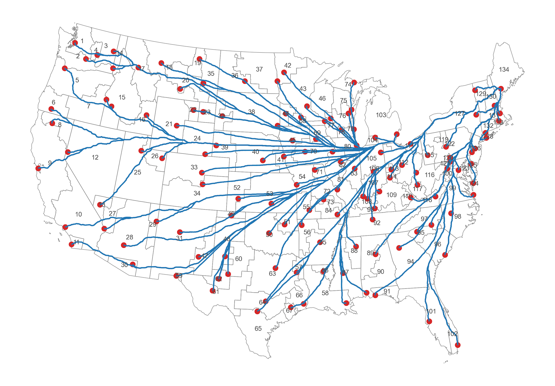
Fig. 50 Example least-cost paths from Maine to each of the other model zones. Least-cost paths are determined between each pair of zones.
By default, endogenous expansion of interzonal transmission capacity is allowed to begin 8 years after the present year. All components and types of interzonal transmission (including both per-mile line costs and AC/DC converters) use a financial multiplier calculated using a 40-year capital recovery period.
Transmission assumptions
These transmission assumptions (and others described below) are controlled by parameters in the inputs/scalars.csv file.
For example:
trans_crp: Capital recovery period for interzonal transmission (default 40 years)years_until_trans_longterm: Years after present until endogenous transmission expansion is allowed (default 8 years).
AC and B2B
New AC transmission capacity uses base costs representative of single-circuit 500-kV lines. By default, interfaces with existing AC capacity can be expanded endogenously. Interfaces crossing between the three asynchronous interconnections that are currently linked by B2B capacity can also be expanded endogenously. B2B connections are modeled as AC lines on either side of an AC/DC/AC converter, so the per-mile costs and distances use AC values. Fig. 51 shows the estimated per-mile interzonal transmission costs for each expandable interface, calculated using the cost surfaces described in Transmission costs and visualized using the least-cost paths described in New transmission capacity.

Fig. 51 Modeled per-mile costs for new AC and B2B transmission additions.
As discussed in Existing transmission capacity, two levels of flow constraints are applied: one at the model zone level and one at the planning subregion level, with existing AC capacity between planning subregions assessed at the \(n - 1\) contingency level. As an approximation of contingency considerations for new transmission capacity (which cannot be assessed directly because interzonal transmission capacity, like all other variables in ReEDS, is represented linearly rather than as individual units or transmission lines), the contribution of new interzonal AC transmission capacity to flow limits between planning subregions is derated by 15%. That is, between a pair of zones that span a planning subregion interface, 100 MW of new interzonal transmission investment increases the flow limit between those two zones by 100 MW but increases the flow limit between the containing planning subregions only by 85 MW. This derate applied only to AC capacity; HVDC capacity between planning subregions (discussed next) is not derated.
Transmission assumptions
The derate on the contribution of new interzonal transmission capacity to flow limits between planning subregions is controlled by the GSw_TransGroupDerate switch in cases.csv.
Within the model, interzonal transmission capacity is represented by the CAPTRAN_ENERGY and CAPTRAN_PRM variables, and AC transmission capacity between planning subregions is represented by the CAPTRAN_GRP variable.
HVDC
Two types of HVDC transmission capacity can be added: point-to-point HVDC connections (assumed to use LCC) and a multiterminal HVDC network (assumed to use VSC) [DOE, 2024]. A schematic overview of these options is provided in Fig. 52.
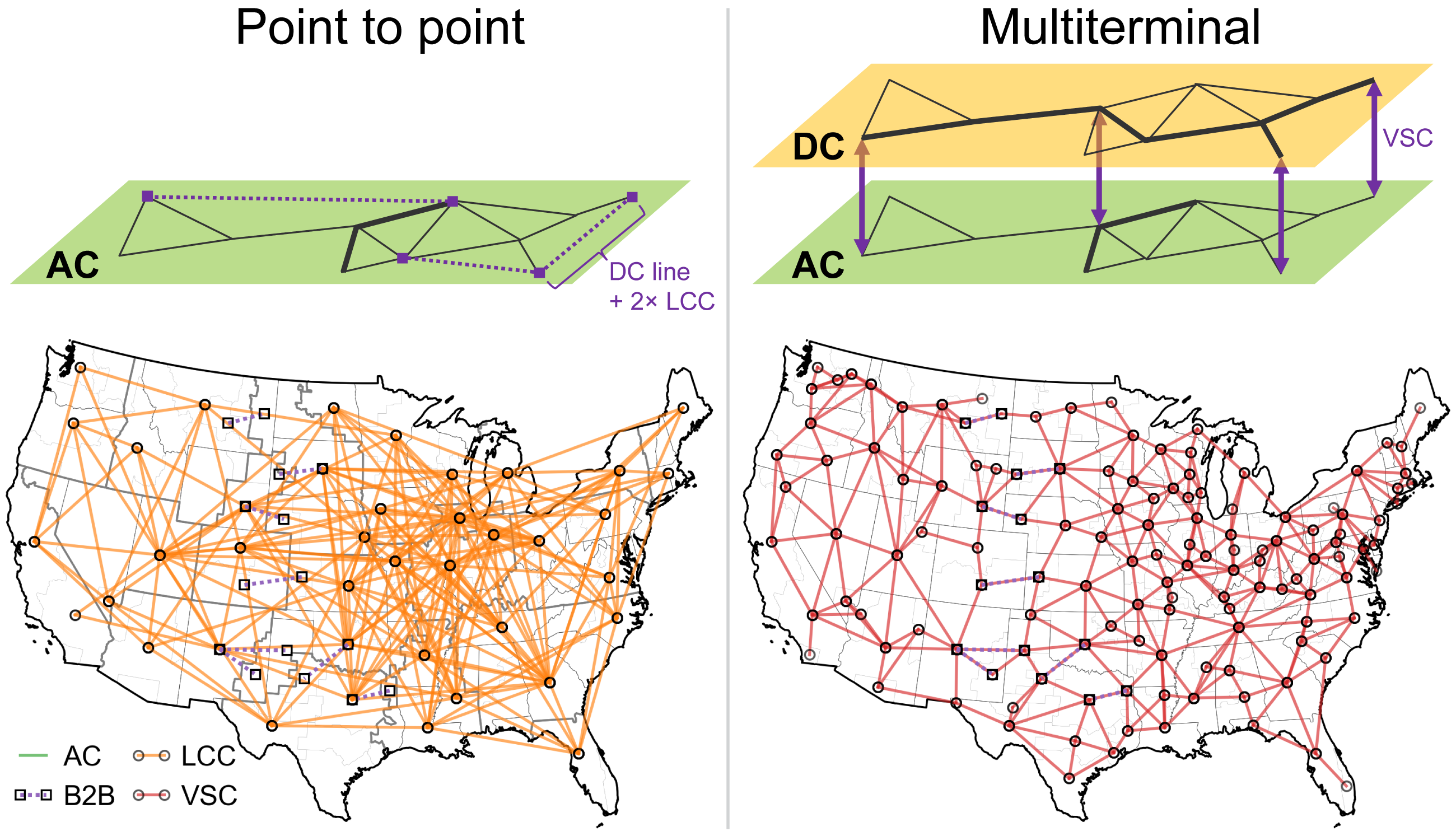
Fig. 52 Schematic overview and example candidate expansion options for point-to-point HVDC (represented as LCC within the model) and multiterminal HVDC (represented as VSC).
Within ReEDS, point-to-point HVDC is represented as part of the AC network, with a converter on either side of the interface; 1 MW of HVDC line capacity is accompanied by 2 MW of converters (1 MW on either side of the interface). If multiple point-to-point HVDC links are added in series—for example, to move power from Zone A to Zone C through an intermediate zone B—AC/DC conversion losses are incurred in each zone. In this three-zone example, adding 1 MW of capacity from Zone A to Zone C would entail adding 1 MW of line capacity to the A-B and B-C interfaces, 1 MW of AC/DC converter capacity in each of Zones A and C, and 2 MW of converter capacity in Zone B.
In the multiterminal HVDC representation, the capacities of HVDC links and AC/DC converters are independently optimized, and the HVDC network is modeled as an “overlay” on top of the AC network, with AC/DC converter capacity linking the two networks. In the three-zone example described in the previous paragraph, adding 1 MW of capacity from Zone A to Zone C under the multiterminal framework would not require any converter capacity to be added in Zone B.
Multiterminal HVDC is turned off by default. Existing HVDC connections (all of which use LCC at the time of this writing) are allowed to be endogenously expanded starting in the same year that new AC capacity additions are allowed.
HVDC scenarios
Additional candidate point-to-point HVDC connections can be allowed using the
GSw_TransScenswitch. For example, the point-to-point connections shown in Fig. 52 can be enabled by settingGSw_TransScen=LCC_1000miles_demand1_wind1_subferc_20230629.Multiterminal HVDC expansion can be turned on by setting
GSw_TransScen=VSC_all.
Losses
Flows over AC and B2B transmission links incur volumetric energy losses of 1% per 100 miles, with the characteristic length of each interface given by the length of the least-cost path described above. Flows over HVDC transmission links incur volumetric energy losses of 0.5% per 100 miles. Additional losses are incurred for HVDC links when energy flows through an AC/DC converter: Losses for LCC are assumed to be 0.7% (for a total of 1.4% losses because two converters are required for each HVDC link), and losses for VSC are assumed to be 1% [Alassi et al., 2019]. B2B connections are modeled as two LCC converters in series and thus incur losses of 1.4%, in addition to length-dependent losses for the AC links on either side of the converters.
Offshore transmission
By default, offshore wind resources are assumed to be connected radially to land-based zones and offshore wind generation is assigned to the associated land-based zone; in this default formulation, offshore-to-land transmission flows are not directly modeled. An alternate formulation adds dedicated offshore zones to the model and explicitly tracks transmission capacity and flows between offshore and land-based zones. Fig. 53 illustrates the offshore zones and associated candidate transmission connections.
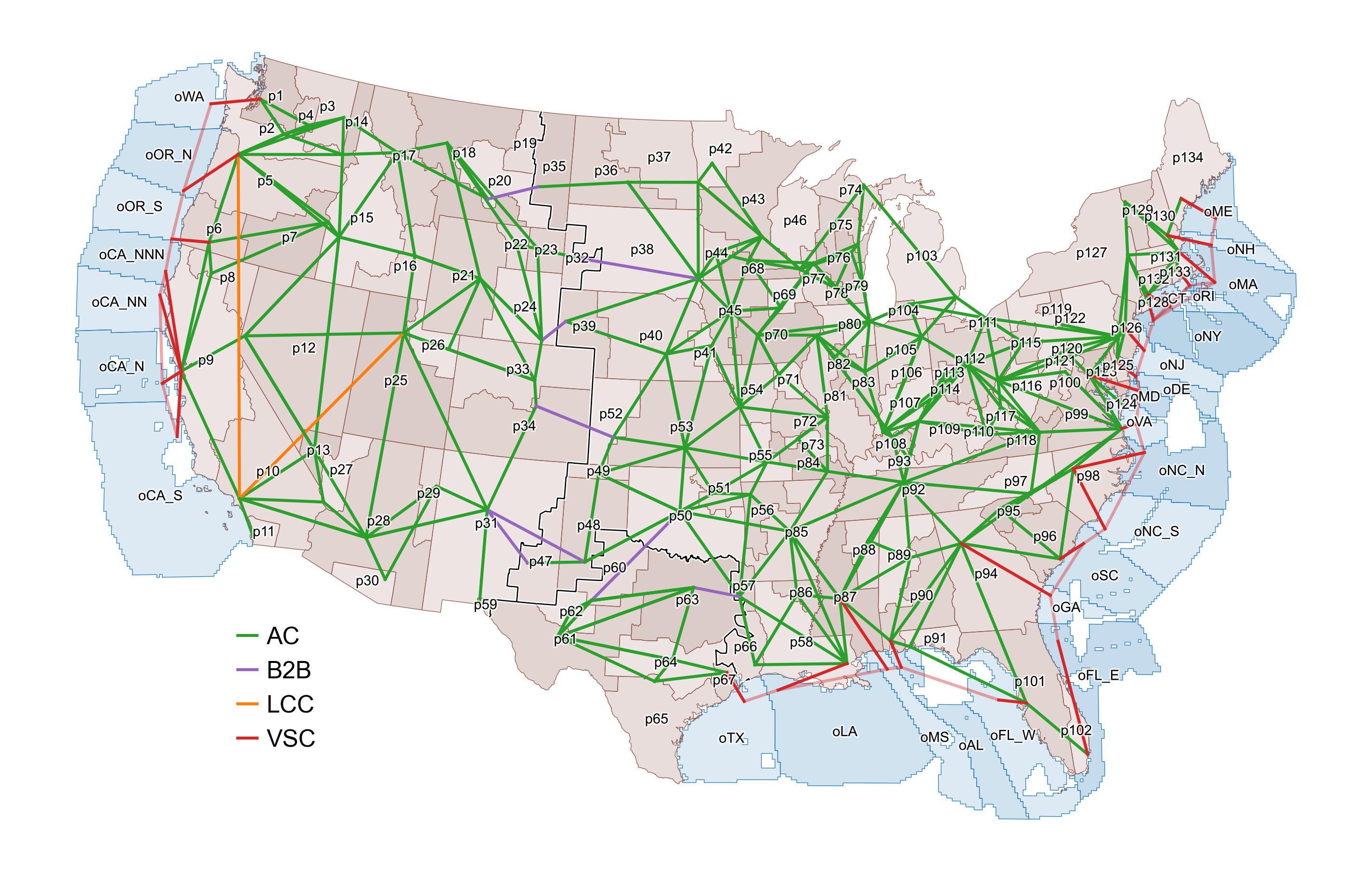
Fig. 53 Default interzonal transmission expansion candidates when offshore zones are enabled.
Offshore zones
The following switches control the representation of offshore zones:
GSw_OffshoreZones(default0): If set to1, offshore zones are turned on; otherwise, if set to0, offshore wind generation is directly assigned to the associated land-based zone.GSw_OffshoreBackbone(default0): If set to1, new transmission capacity may be added between offshore zones, enabling the construction of offshore transmission “backbones”. These “backbone” links are shown in light red in Fig. 53; radial links between offshore and land-based zones are shown in darker red. IfGSw_OffshoreBackboneis set to0, only the darker red radial links may be built.GSw_OffshoreBackflow(default0): If set to1, transmission flows from land-based zones to offshore zones are allowed; when combined withGSw_OffshoreBackbone, this switch allows offshore transmission to be built and operated independently of offshore wind (for example, to bypass high-cost land-based transmission routes). IfGSw_OffshoreBackflowis set to0, transmission flows from land to offshore zones are not allowed.
Hurdle Rates
ReEDS includes a default hurdle rate of $0.01/MWh (in 2004$) to reduce degeneracy by marginally incentivizing local energy consumption over interzonal energy trades.
Higher hurdle rates, although not turned on by default, can also be used. Different hurdle rates can be applied at different levels of the regional structure shown in Fig. 18. For example, a higher hurdle rate can be applied to flows between planning regions than to flows within planning regions.
Hurdle rates
Higher hurdle rates can be turned on by setting GSw_TransHurdleRate=1.
When this setting is activated, the hurdle rate for flows between planning subregions starts at 8 $2020/MWh [John Tsoukalis et al., 2020] and linearly declines to half of that value between 2026 and 2050.
The hurdle rate for flows between hurdle regions (Fig. 18) starts at the same value but declines to zero by 2050.
Within hurdle regions, only the nominal $0.01/MWh hurdle rate is applied.
These region boundaries can be changed using the GSw_TransHurdleLevel1 and GSw_TransHurdleLevel2 switches.
International Electricity Trade
ReEDS represents electricity trade with Canada exogenously. (Electricity trade with Mexico is not represented.) In the default configuration, imports and exports are specified by Canadian province based on the Canada Energy Regulator Canadian Electricity Futures 2023 Current Measures [Canada Energy Regulator, 2023], with net exports across all regions shown in Fig. 54. Each province is required to send electricity to or receive electricity from any of the ReEDS zones that have connecting transmission lines to that province, with the split among zones approximated based on the transmission connecting the zones to the provinces. Seasonal and time-slice estimates for imports and exports are based on the historical monthly flows between the countries [Canada Energy Regulator, 2024]. Canadian imports are assumed to be from hydropower and are counted toward RPS requirements where allowed by state RPS regulations. Canadian imports also count toward reserve margin requirements.
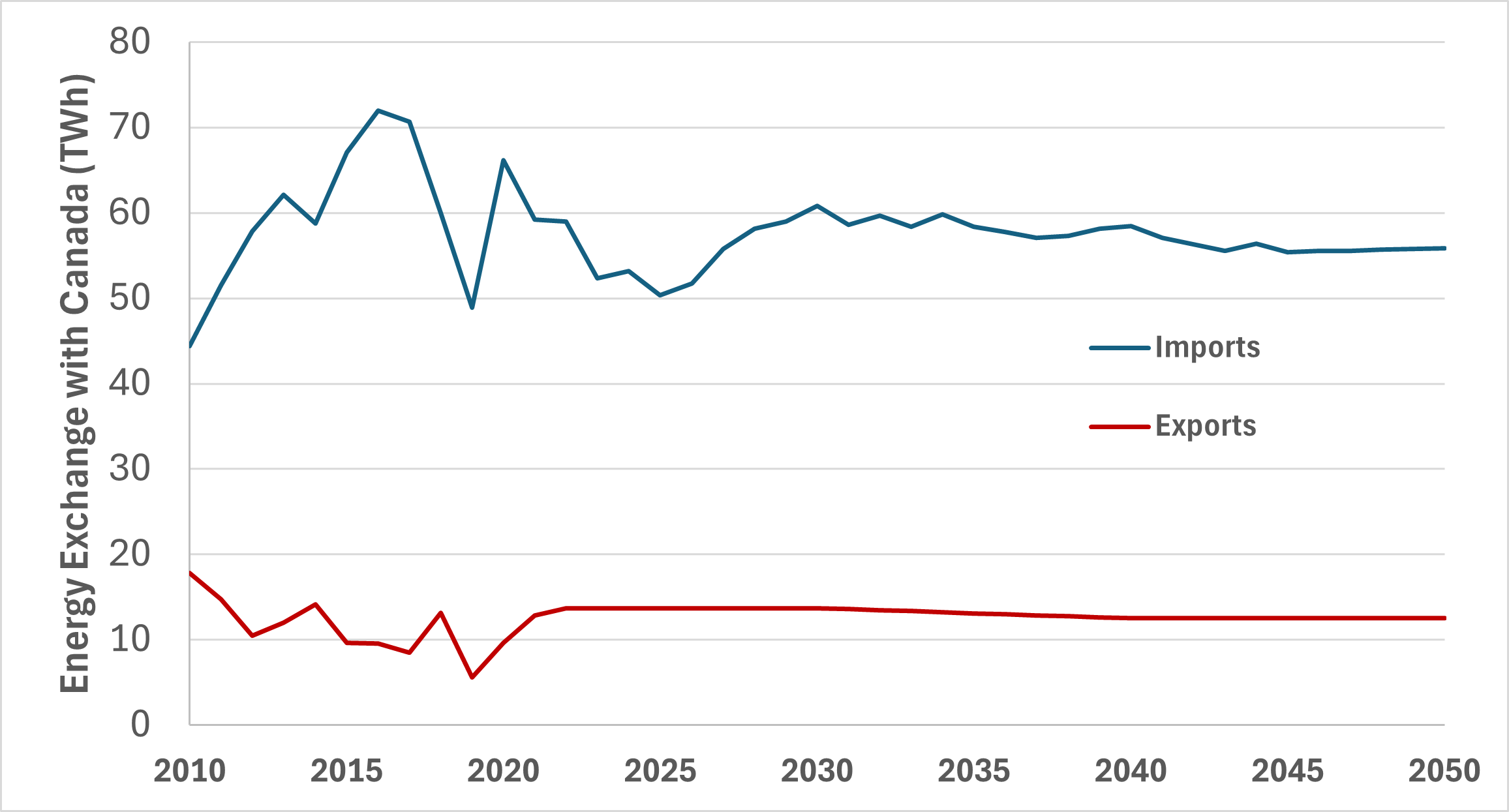
Fig. 54 Imports from Canada to the United States and exports from the United States to Canada.
Electricity System Operation and Reliability
ReEDS finds the least-cost way to build and operate the electricity system while meeting certain requirements that are dominated by the need to meet electricity load while maintaining system adequacy and operational reliability.
Supply/Demand Balance
Electricity demand is required to be met in each modeled time step and model zone. The end-use electricity load projection used in ReEDS is exogenously defined. There are many exogenous load profiles available in the model, designed to accommodate various study needs and sensitivities. Especially as the electrification of nonelectric energy uses creates significant regional and temporal shifts to the electric sector load representation, the choice of load profile is important because it contributes to the technology deployment mix and quantity.
The ReEDS load profiles are at hourly zonal resolution. However, their sources and processing through the model vary slightly, as described in the following subsections.
Operational Reliability
In addition to ensuring adequate capacity to satisfy long-term planning reserve requirements, ReEDS requires operational reliability—that is, the ability to continue operating the bulk power system in the event of a sudden disturbance [NERC, 2016]. In practice, ancillary reserve requirements ensure there is sufficient flexibility from supply-side and demand-side technologies to rebalance fluctuations in generation and demand.
ReEDS represents three types of operating reserve products: spinning, regulation, and flexibility reserves [Cole et al., 2018]. The requirement specified for each product in each time slice is a function of load, wind generation, and photovoltaic capacity (during daytime hours).[24] Technologies providing these reserve products must be able to ramp their output within a certain amount of time. ReEDS can also represent a “combo” reserve product that combines the three operating reserve products into a single hybrid product. The “combo” approach is used to reduce model size and improve runtime.
Operating reserve requirements are summarized in Table 13, with data taken from [Lew et al., 2013]. The flexibility requirement for wind is estimated as the ratio of the change in the reserve requirement to the change in wind generation from the High Wind scenario in [Lew et al., 2013]; the requirement was estimated similarly for PV using the High Solar scenario in [Lew et al., 2013]. The estimated regulation requirements (0.5% wind generation and 0.3% PV capacity) are based on incremental increases in regulation reserves across all scenarios in [Lew et al., 2013].
Reserve Product |
Load Requirement (% of load) |
Wind Requirement (% of generation) |
PV Requirement (% of capacity [AC]) |
Time Requirement to Ramp (minutes) |
|---|---|---|---|---|
Spinning |
3% |
— |
— |
10 |
Regulation |
1% |
0.5% |
0.3% |
5 |
Flexibility |
— |
10% |
4% |
60 |
All ancillary reserve requirements must be satisfied in each zone for each time slice; however, reserve provision can be traded between zones using AC transmission interfaces. Trades are allowed only within planning regions (Fig. 18) and not across planning region boundaries. The amount of reserves that can be traded is limited by the amount of carrying capacity of an AC transmission interface that is not already being used for trading energy.
The ability of technologies to contribute to reserves is limited by the ramping requirement for a given reserve product, the plant ramp rate, and online capacity (Table 14). Online capacity is approximated in ReEDS as the maximum generation from all time slices within a modeled day. Reserves can be provided by generation and storage technologies that are turned on but not fully dispatched in a time slice. In addition, demand-side interruptible load can also contribute to reserve requirements, if enabled in a scenario. PV and wind are not allowed to contribute toward the supply of reserves.
The cost for providing regulation reserves is represented in ReEDS using data from [Hummon et al., 2013]; see Table 15. Because ReEDS does not clearly distinguish between coal fuel types, $12.5/MWh is the assumed regulation cost for all coal technologies. The cost of providing regulation reserves from gas-CT, geothermal, biopower, and landfill gas is assumed to be the same as oil/gas steam.
Assumed Ramp Rate (%/min) |
Upper Bound (% of online capacity) = Ramp Rate (%/min) × Ramp Requirement (min) |
|||
|---|---|---|---|---|
Spinning |
Regulation |
Flexibility |
||
Gas-CTa |
8 |
8×10=80 |
8×5=40 |
8×60=480, so 100 |
Gas-CCa |
5 |
5×10=50 |
5×5=-25 |
5×60=300, so 100 |
Coala |
4 |
4×10=40 |
4×5=20 |
4×60=240, so 100 |
Geothermalb |
4 |
4×10=40 |
4×5=20 |
4×60=240, so 100 |
CSP with Storagec |
10 |
10×10=100 |
10×5=50 |
10×60=600, so 100 |
Biopowerb |
4 |
4×10=40 |
4×5=20 |
4×60=240, so 100 |
Oil/Gas Steama |
4 |
4×10=40 |
4×5=20 |
4×60=240, so 100 |
Hydropower |
100 |
No Upper Bound |
No Upper Bound |
No Upper Bound |
Storage |
100 |
No Upper Bound |
No Upper Bound |
No Upper Bound |
a See [Bloom et al., 2016]. b Geothermal and biopower values are assumed to be the same as oil/gas steam units. In practice, geothermal plants typically do not ramp given their zero or near-zero variable costs and therefore provide only energy and not operating reserves. c. See [Jorgenson et al., 2013].
Generator Type |
Cost of Regulation Reserves (2013$/MWh) |
|---|---|
Supercritical Coal |
15 |
Subcritical Coal |
10 |
Combined Cycle |
6 |
Gas/Oil Steam |
4 |
Hydropower |
2 |
Pumped Storage Hydropower |
2 |
Because stress periods already hold an hourly amount of reserves, it overlaps with the operating reserves and renders them unnecessary. Therefore, operating reserves are typically turned off when using the stress period formulation.
Resource Adequacy
Resource adequacy (RA) is defined by the North American Electric Reliability Corporation as “[t]he ability of the electric system to supply the aggregate electric power and energy requirements of electricity consumers at all times while taking into account scheduled and reasonably expected unscheduled outages of system components” [NERC, 2022]. ReEDs users can select between two RA modeling methods, illustrated graphically in Fig. 55. In the default “stress periods” method, additional periods (typically days) with a higher risk of unserved energy—referred to here as stress periods—are modeled alongside the representative periods described in the Temporal Resolution section; the linked Probabilistic Resource Adequacy Suite (PRAS) model [Stephen, 2021] is run after each ReEDS model year to evaluate the RA of the ReEDS-designed power system and add additional stress periods if necessary. In the “capacity credit” method, ReEDS instead enforces a seasonal firm capacity constraint, with the capacity credit of variable renewable energy and storage technologies calculated using net load profiles between each pair of ReEDS model years. The stress periods method captures the combined capacity value of generation, storage, and interregional transmission, accounting for the energy availability of all resources, and approximates suggested best practices [Carvallo et al., 2023, Stenclik, 2023]; the capacity credit method is more reflective of current practice in many jurisdictions. These methods are described in more detail below.
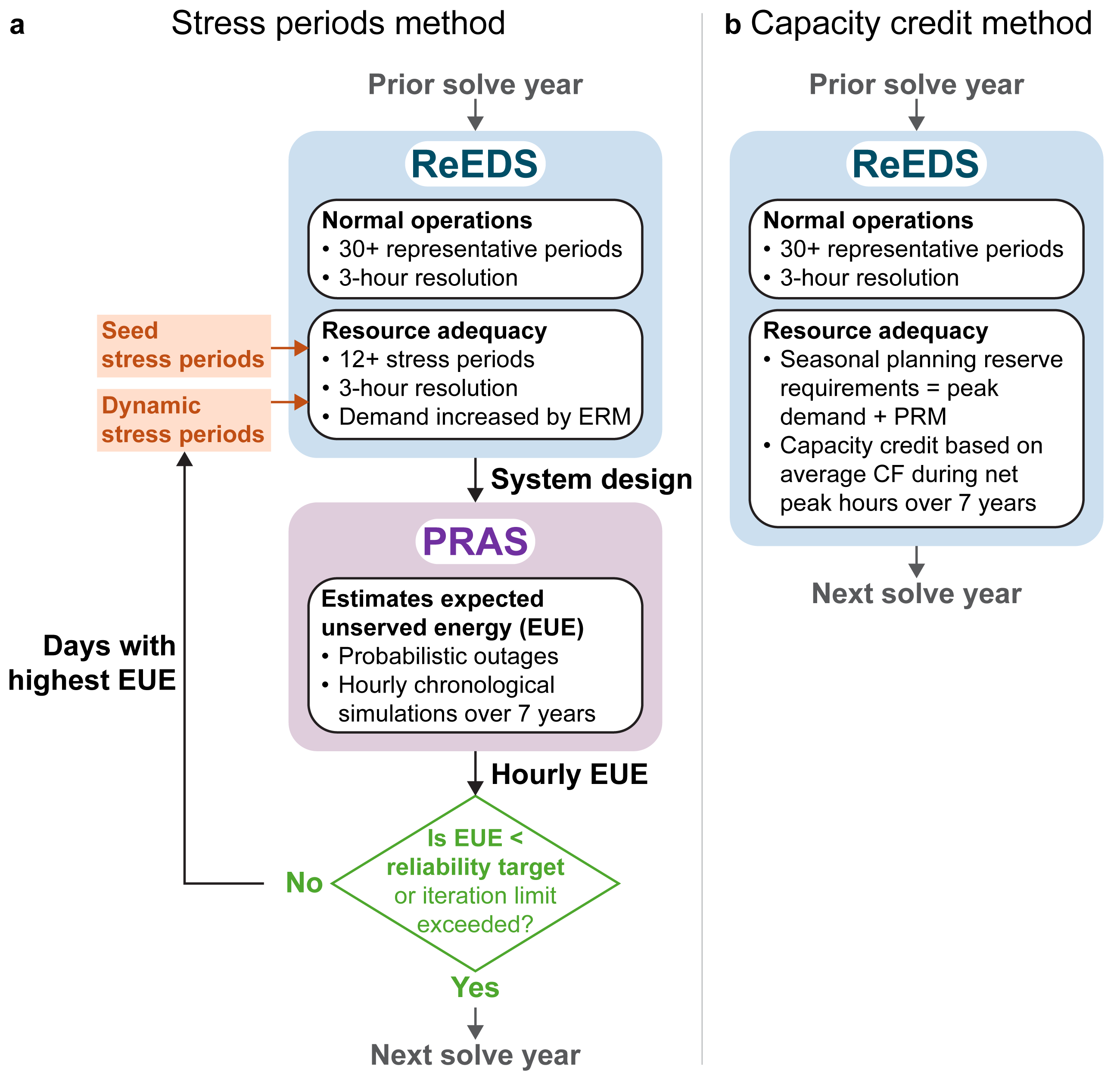
Fig. 55 Model flow for the stress periods (a) and capacity credit (b) methods. Adapted from [Mai et al., 2024].
“Stress Periods” RA Method
The stress periods method is described in detail by [Mai et al., 2024]. Within the ReEDS optimization, stress periods are modeled in the same manner as representative periods (using the same sets of variables and constraints for storage operations, transmission flows, and VRE availability, for example), with the following exceptions:
Electricity demand during stress periods is scaled up by the planning reserve margin.
The “weight” of stress periods (used in the calculation of operational costs including fuel costs, VOM costs, etc.) is set to 6 hours in total per year. Representative periods, in contrast, are weighted at 8760 hours per year (for an average of 365.25 days per year, accounting for leap years). This approach—with a low but nonzero weight during stress periods—provides realistic dispatch profiles during stress periods but ensures reported operational costs are dominated by the representative periods, which are selected to minimize regional errors in electricity demand and capacity factor associated with time series aggregation.
Hydrogen fuel is assumed to be always available during stress periods; stress periods are not part of the interday accounting of hydrogen storage levels shown in Fig. 23, and endogenous electricity demand from electrolyzers, steam methane reforming, and DAC is assumed to be zero during stress periods.
Diurnal storage (batteries and pumped hydro) is modeled continuously over chronologically consecutive stress periods; for example, if both 2008-02-27 and 2008-02-28 are stress periods, the last hour of 2008-02-27 links to the first hour of 2008-02-28, and the last hour of 2008-02-28 links back to the first hour of 2008-02-27. If a stress period has no consecutively adjacent stress periods, it is modeled with periodic boundary conditions linking the last hour of the period to the first hour of the same period (the same treatment as representative periods, as long as interday storage operation is not enabled).
Interregional transmission flows are allowed during stress periods by default, allowing interregional coordination to help meet resource adequacy needs. New transmission capacity is derated by 15% during stress periods to approximate contingency considerations.
Coincident net imports into NERC regions (Fig. 18) during stress periods are by default limited to historical peak net firm capacity transfers from [NERC, 2023] through 2030 to approximate barriers to coordinated interregional resource adequacy planning.
“Seed” stress periods
As shown in Fig. 55, the iterative ReEDS-PRAS procedure begins with a set of “seed” stress periods for each model year. Seed stress periods are included because representative periods do not, in general, include outlying periods (such as peak demand days) that drive capacity investments. A system planned only with representative periods would therefore almost certainly fail to meet resource adequacy targets when considering a broader collection of weather and demand conditions, and the inclusion of seed stress periods allows this initial failing iteration to be skipped, reducing runtime.
By default, seed stress periods include peak demand days by planning subregion for each model year, in addition to minimum availability days for solar and wind by interconnection (shown in Fig. 56 for an illustrative high-electrification scenario).
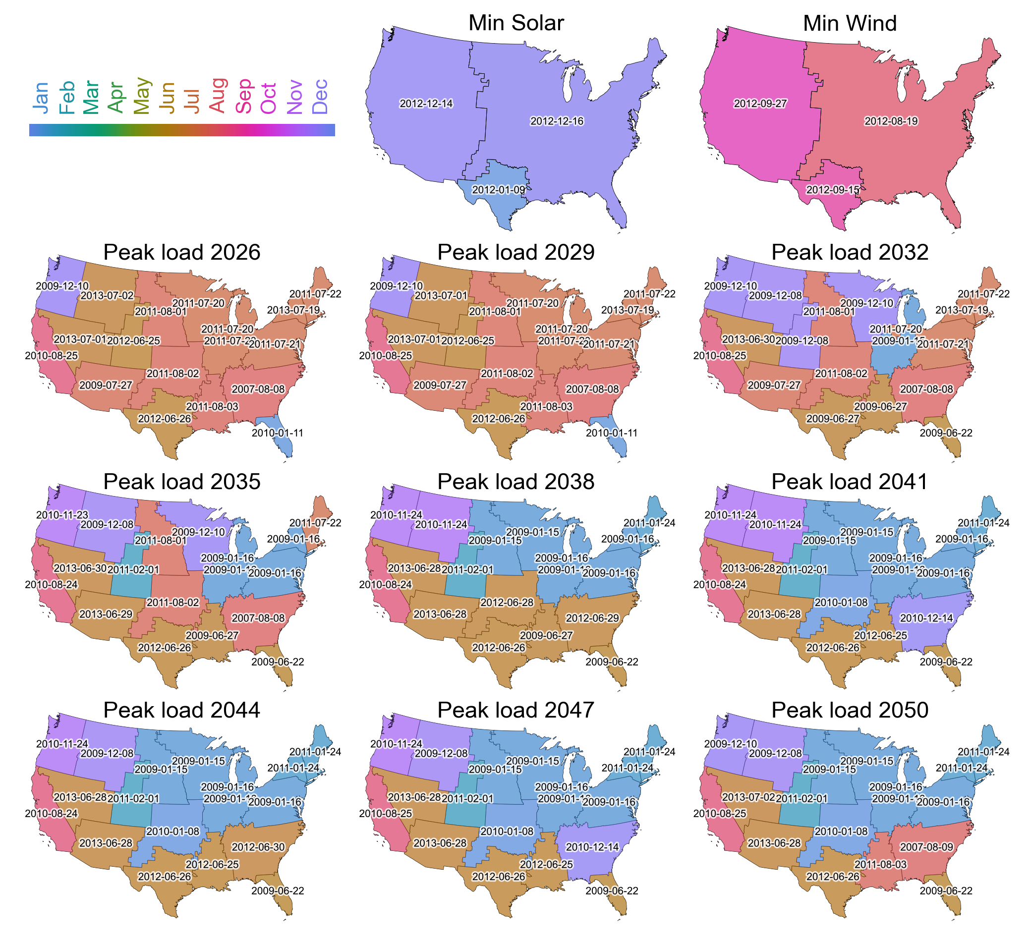
Fig. 56 Example “seed” stress periods for a high-electrification scenario. In this scenario, many regions in the northern half of the country switch from summer peaking to winter peaking by midcentury.
ReEDS2PRAS
After each model year is optimized in the capacity expansion model, the resulting electricity system design is passed to PRAS for resource adequacy assessment. This model-to-model translation is performed by the “ReEDS2PRAS” submodule. PRAS, described in detail by [Stephen, 2021], models individual unit outages using a two-state Markov model with Monte Carlo sampling; by default, the application of PRAS in the coupled ReEDS-PRAS model uses chronological hourly resolution over seven weather years (2007–2013).
ReEDS2PRAS converts the modeled system from the linear generation and storage capacities used in ReEDS to the individual units considered in PRAS, making the following assumptions (some of which can be changed by the user):
Thermal generation
Existing thermal generation capacity is disaggregated using unit sizes from the EIA-NEMS database of existing units (Fig. 36) [EIA, 2025].
Unit sizes for new thermal generation capacity depend on whether the model zone hosts existing capacity of that technology type and on the planning reserve margin of the model zone. Remainder capacity is assigned to its own unit (so 210 MW of capacity, with a 100 MW unit size, would be disaggregated into 3 = 2 × 100 MW + 1 × 10 MW units).
If existing units are present, the average of the existing unit sizes is used for newly added capacity.
If no existing units are present, the assumed unit size from [NREL, 2024] is used for newly added capacity. These unit sizes are shown in Table 16.
The unit size described in the previous bullets is capped at the zonal planning reserve margin in MW (given by the zonal peak demand [MW] multiplied by the fractional planning reserve margin). For example, if a zone has a peak demand of 1000 MW and a 15% planning reserve margin, the maximum size for new units is 150 MW; if ReEDS sites 460 MW of gas-CT (with a characteristic unit size of 233 MW) in this zone, this capacity would be disaggregated into four (3 × 150 MW + 1 × 10 MW) units instead of two (1 × 233 MW + 1 × 227 MW). This condition helps mitigate the \(n - 1\) contingency risk that would result from using unit sizes larger than the reserve margin.
Hourly temperature-dependent forced outage rates (FOR; shown in Fig. 39) and mean time to repair (MTTR; shown in Table 16) are converted to hourly failure (\(\lambda\)) and recovery (\(\mu\)) probabilities using the following equations:
\(\mu = \frac{1}{\text{MTTR}}\)
\(\lambda = \frac{\mu \cdot \text{FOR}}{1 - \text{FOR}}\)
VRE (wind and solar)
Average outage rates are already included in the hourly capacity factor profiles for VRE used throughout ReEDS and PRAS, so VRE capacity is not disaggregated in ReEDS2PRAS and unit outages are not modeled using the Monte Carlo approach applied for thermal generators. Extreme-cold and icing-related outages for wind are also included in the hourly capacity factor profiles used throughout both models (Fig. 42).
Energy storage
Battery installations are not disaggregated into individual units, and outages are not modeled probabilistically. This simplification is made to reduce runtime; because battery installations are modular with relatively small units, modeling unit outages for batteries would dramatically increase the number of units and reduce model performance.
Pumped hydro installations are disaggregated in the same manner as thermal generation, with unit sizes based on existing regional unit sizes or ATB assumptions.
Transmission
Transmission outages are not considered in ReEDS2PRAS, and PRAS uses the same “pipe and bubble” approximation for transmission flow as ReEDS.
Technology |
Max Unit Capacity [MW] |
Mean Time To Repair [hours] |
|---|---|---|
Nuclear |
1,117 |
298 |
Pumped hydro |
1,000 |
24 |
Combined cycle |
727 |
48 |
Coal, nonintegrated gasification and combined cycle (IGCC) |
650 |
55 |
Coal, IGCC |
634 |
55 |
Combustion turbine (fossil gas and H2) |
233 |
48 |
Oil-gas-steam |
233 |
48 |
Hydropower |
94 |
24 |
Biopower and landfill gas |
50 |
38 |
Geothermal |
30 |
24 |
Fig. 57 shows an example distribution of thermal and hydro unit capacities generated by ReEDS2PRAS.
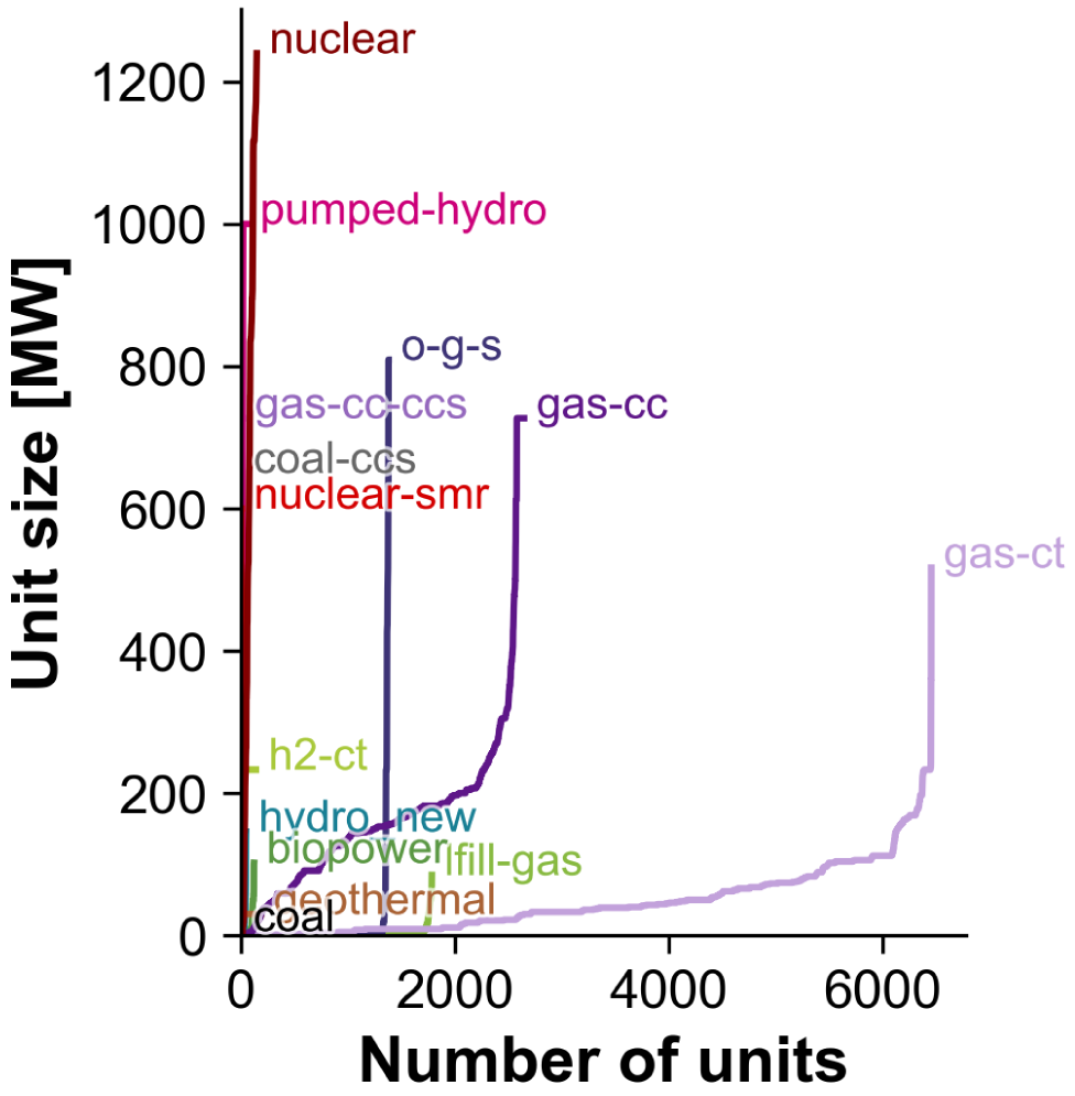
Fig. 57 Unit capacity distribution generated by ReEDS2PRAS for an illustrative scenario and model year.
Iteration between ReEDS and PRAS
The PRAS model calculates (among other quantities) the hourly expected unserved energy (EUE) in each model zone across a user-defined number of Monte Carlo samples (10 samples by default). The hourly EUE profiles are summed at the resolution used for RA assessment (the 18 planning subregions by default) and divided by total electricity demand to determine the normalized EUE (NEUE). The NEUE in each region is then compared to the user-specified reliability threshold; if any regions do not meet the specified threshold, the days with highest EUE in the failing regions are added as “dynamic” stress periods (Fig. 55) and another ReEDS-PRAS iteration is performed. This process is illustrated graphically in Fig. 58. Once all regions meet the reliability threshold (or once a user-specified maximum number of iterations is reached), the simulation progresses to the next model year, and the process begins again (Fig. 17). The default reliability threshold of 1 ppm NEUE is roughly equivalent to a loss of load expectation of 0.1 days/year in many regions [EPRI, 2024].
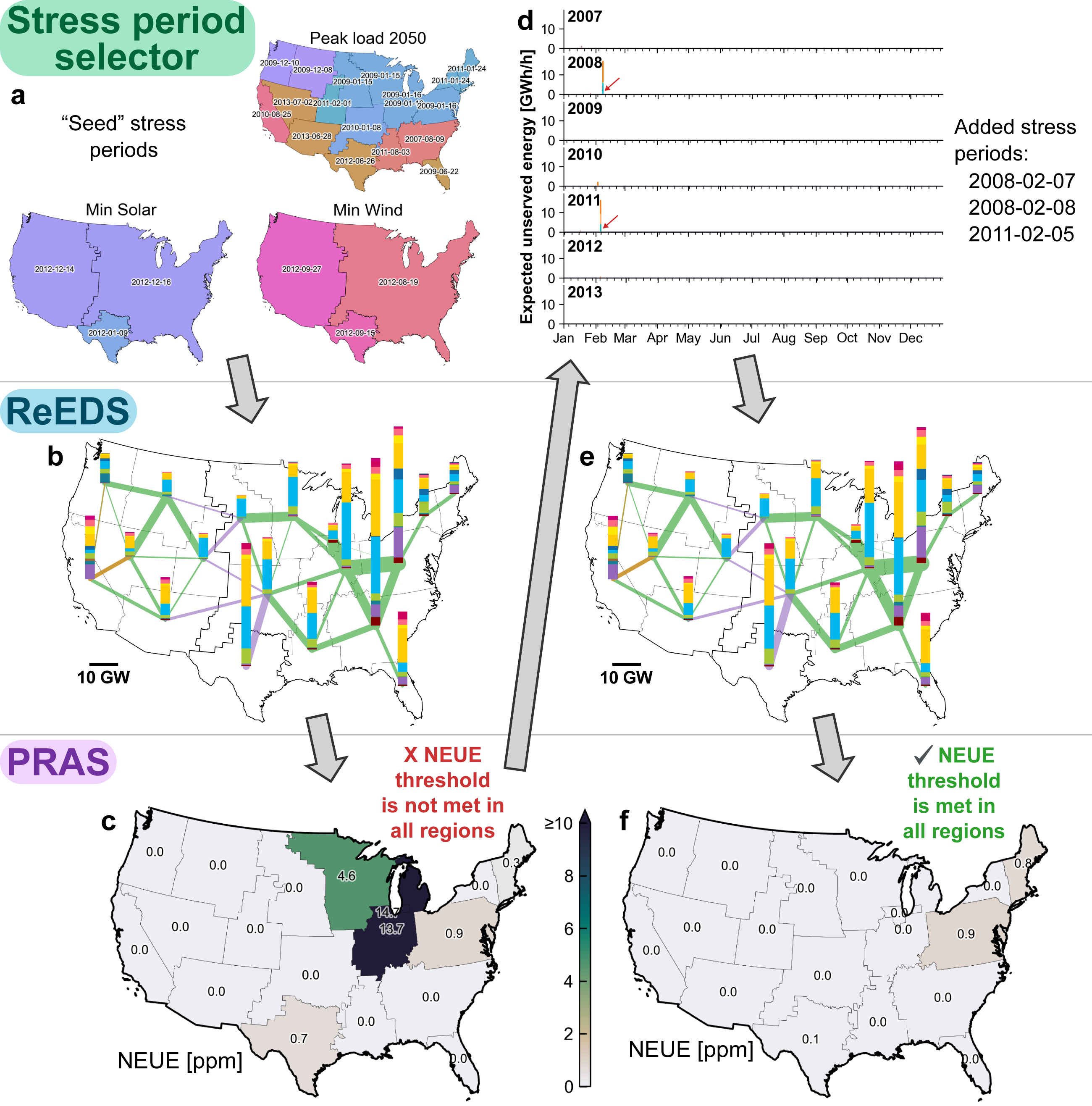
Fig. 58 Iterative capacity expansion and resource adequacy model flow for an illustrative scenario, reproduced from [Mai et al., 2024]. a, “Seed” stress periods. b, ReEDS capacity expansion results for the first iteration using only the “seed” stress periods. Actual results are at zonal resolution but are aggregated here to the level of the 18 planning subregions (Fig. 18) for clarity. c, Regional NEUE determined by PRAS for the ReEDS system shown in b. Some regions do not meet the 1 ppm NEUE threshold, triggering a second iteration in the process. d, Hourly expected unserved energy (EUE) for the 2007–2013 weather years as determined by PRAS. The 3 days listed are added as new stress periods for the next iteration. e, ReEDS capacity expansion results using the added stress periods, and f, PRAS NEUE for the second-iteration system. All regions meet the 1 ppm NEUE target, so the process is complete for the present model year.
Fig. 59 shows the evolution of NEUE over successive ReEDS-PRAS iterations for an illustrative ReEDS scenario. The “seed” stress periods in iteration 0 are the same as in Fig. 56. In this example, most years are resource-adequate with the “seed” stress periods alone; years 2032, 2035, and 2044 require one extra ReEDS-PRAS cycle to add additional stress periods because the first iteration does not meet the 1 ppm NEUE threshold in all planning subregions.
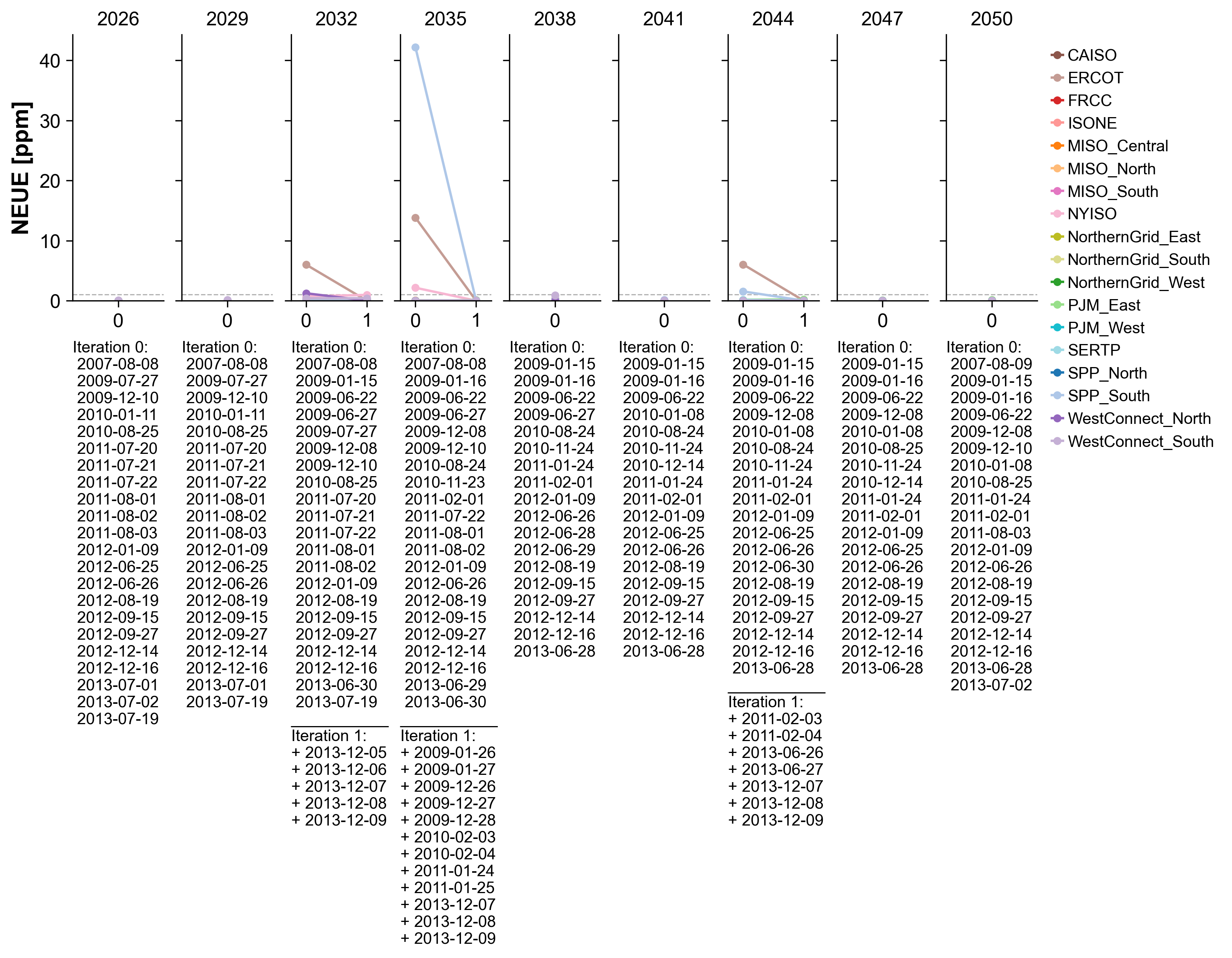
Fig. 59 Evolution of stress periods for an illustrative ReEDS scenario.
Resource adequacy settings
Model settings related to resource adequacy can be adjusted by the user using switches in the cases.csv file.
The syntax for these switches is described in the “Description” column of cases.csv, and their operation is briefly outlined below.
Choose between stress periods vs. capacity credit
GSw_PRM_CapCredit(default 0): Use stress periods if 0, capacity credit if 1
Control the iteration between ReEDS and PRAS
GSw_PRM_StressThreshold(defaulttransgrp_10_EUE_sum): Regional RA threshold for stress period iterationGSw_PRM_StressIterateMax(default 5): Max number of times to iterate on a particular solve yearGSw_PRM_StressIncrement(default 2): How many stress periods to add per region per iterationGSw_PRM_StressStorageCutoff(defaultEUE_0.1): How to select “shoulder” stress periods for interday storageGSw_PRM_StressModel(defaultpras): Interface for specifying fixed user-defined stress periods; when set topras, stress periods are identified dynamically
Specify how “seed” stress periods are defined
GSw_PRM_StressSeedLoadLevel(defaulttransgrp): Region hierarchy level for peak load “seed” stress periodsGSw_PRM_StressSeedMinRElevel(defaultinterconnect): Region hierarchy level for min-PV/wind “seed” stress periods
Control interregional resource adequacy coordination / firm capacity trading
GSw_PRMTRADE_level(defaultcountry): Region hierarchy level within which to allow firm capacity tradingGSw_PRM_NetImportLimit(default 1): Turn on (1) / off (0) constraint on net firm importsGSw_PRM_NetImportLimitScen(default2031_hist/2050_100): Specify net firm import limit scenarioGSw_TransInvPRMderate(default 0.15): Fractional amount by which to derate the capacity of new transmission for firm capacity trading
Specify the assumed evolution of the planning reserve margin (PRM) across regions
GSw_PRM_scenario(default 0.12): Scenario specifying assumed PRM levels by NERC region and year
Additional RA modeling details
resource_adequacy_years(default2007_2008_2009_2010_2011_2012_2013): Weather years to include in resource adequacy calculationsGSw_HourlyChunkLengthStress(default 3): Hours per time chunk modeled during stress periodspras_samples(default 10): Number of Monte Carlo outage draws modeled in PRASGSw_PRM_StressLoadAggMethod(defaultmax): How to aggregate load within time chunks: “mean” or “max”GSw_PRM_StressOutages(default 1): Turn on (1) / off (0) outages during stress periods in ReEDS
Capacity Credit RA Method
In the capacity credit method, resource adequacy is enforced by requiring the system to have sufficient “firm capacity” to meet the forecasted peak demand plus a planning reserve margin, where the “firm capacity” contributed by each technology is given by the product of that technology’s nameplate capacity and its “capacity credit.” The capacity credit reflects each technology’s expected availability during peak and net-peak hours, where net-peak demand is demand minus VRE generation. The firm capacity constraint is enforced seasonally, and seasonal capacity credits for VRE and storage are calculated regionally between each pair of model years using multiple weather years; capacity credit changes over time as demand and net-demand patterns change, as shown in Fig. 60.
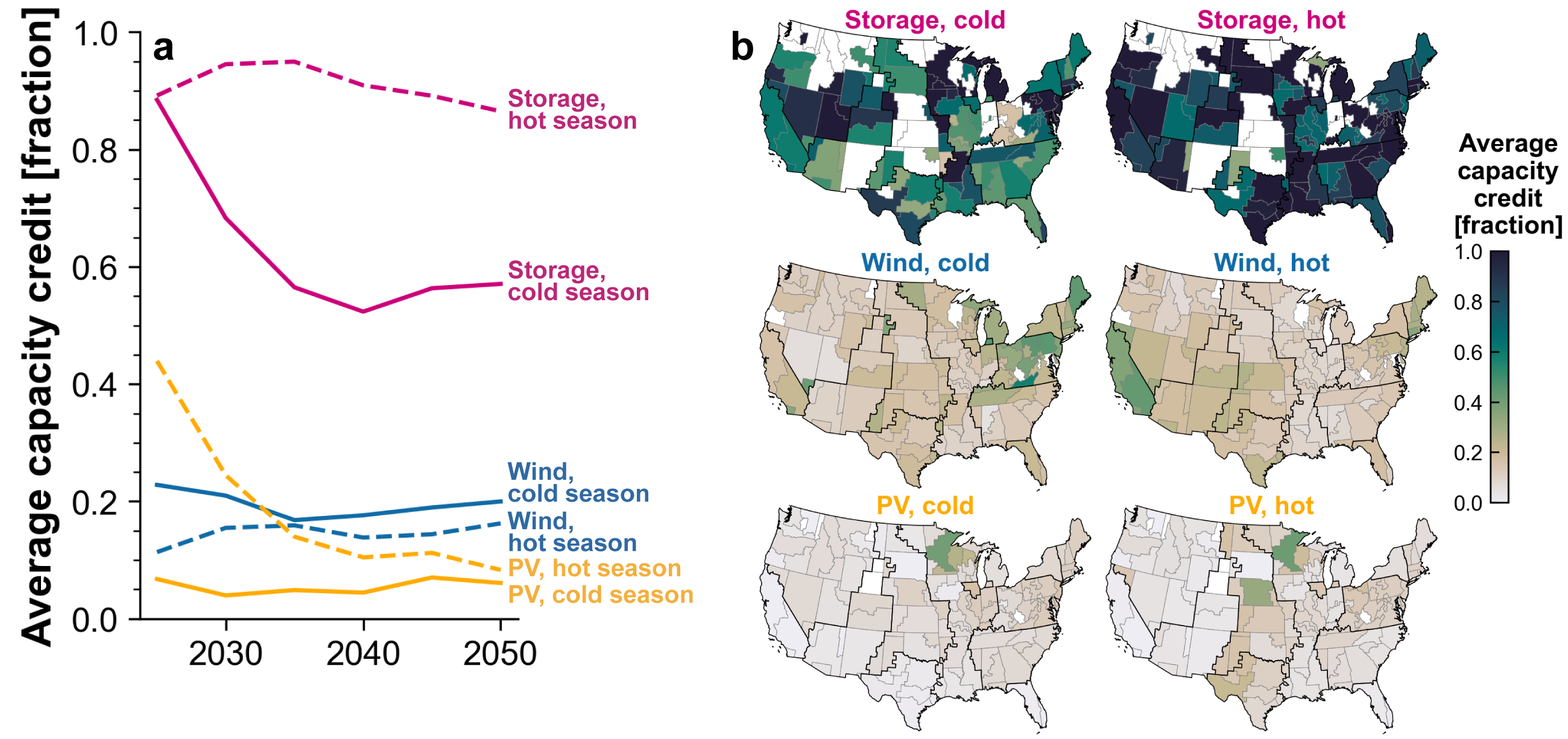
Fig. 60 VRE and storage capacity credit for an illustrative scenario, illustrating yearly and seasonal changes in response to changing system conditions (a) and regional resolution for the values in 2050 (b). White areas in b have no installed capacity of the indicated technology in 2050 in this scenario. Adapted from [Mai et al., 2024].
The calculation of capacity credit for VRE is described in the VRE capacity credit section; the method for storage is described in the storage capacity credit section. Thermal generators are given a capacity credit of 100% in ReEDS; technology-specific outage rates for thermal generators are not considered in this method and are instead assumed to be factored into the planning reserve margin.
VRE capacity credit
For VRE technologies (i.e., wind and solar), ReEDS estimates a seasonal capacity credit for each region/class combination via an hourly LDC approximation of effective load carrying capability (ELCC)[25] performed between solve years. ELCC can be described as the amount of additional load that can be accommodated by adding those generators while maintaining a constant reliability level. The “8760-based” methodology can capture the highest load and net load hours, which typically represent the highest-risk hours, and can thereby support a reasonable representation of capacity credit. Details of this LDC approach as well as a comparison against a former statistical method can be found in [Frew et al., 2017], although that approach has been expanded to consider multiple weather years of wind, solar, and load data rather than just a single year.
The LDC approach for calculating capacity credit is based on explicit hourly tracking of time-synchronous load and VRE resources. The capacity credit method uses a capacity factor proxy that is applied to the top 20 hours (by default) in load and net load-duration curves (LDCs and NLDCs) in each season to estimate ELCC by season. Fig. 61 graphically represents the ReEDS capacity credit methodology. The LDC reflects the total load in a given modeling region, which is sorted from the hours of highest load to lowest load and is shown by the blue line. The NLDC represents the total load minus the time-synchronous contribution of VRE, where the resulting net load is then sorted from highest to lowest, as shown by the solid red line.[26] The NLDC(δ), which represents further addition of VRE resources, can be created by subtracting the time-synchronous generation of an incremental capacity addition from the NLDC, where the resulting time series is again sorted from highest to lowest; this is shown by the dashed red line.
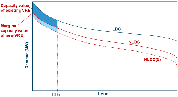
Fig. 61 LDC-based approach to calculating CV.
ReEDS calculates the ELCC as the difference in the areas between the LDC and NLDC during the top 20 hours of the duration curves in each season, as represented by the dark blue shaded area in Fig. 61. These 20 hours are a proxy for the hours with the highest risk for loss of load (i.e., the loss of load probability). Similarly, the contribution of an additional unit of capacity to meeting peak load is the difference in the areas between the NLDC and the NLDC(δ), as shown by the light blue shaded area in Fig. 61. To ensure resource adequacy, ReEDS calculates capacity credit based on a 1,000-MW incremental capacity size of new solar and wind builds. These areas are then divided by the corresponding installed capacity and number of top hours to obtain a fractional seasonal-based capacity credit.
The resulting existing and marginal capacity credit[27] values then feed into ReEDS to quantify each VRE resource’s capacity contribution to the planning reserve requirement. Existing VRE capacity credit calculations are performed by region and technology. For all candidate VRE resources that might be built in the coming year, the marginal capacity credit is calculated by region, technology, and resource class. In all cases, the VRE profile is compared against the aggregated regional load profile for determining the capacity credit (Fig. 61).
Capacity credit settings
Many settings related to capacity credit calculations can be adjusted by the user.
capcredit_hierarchy_level(defaulttransregfor the 11 planning regions shown in Fig. 18): Level at which to aggregate net load for capacity credit calculationGSw_PRM_CapCreditHours(default 20): Number of peak net load hours per capacity credit season considered in capacity credit calculationmarg_vre_mw(default 1000): Amount of marginal VRE capacity to add in MW for marginal capacity credit calculationmarg_stor_mw(default 100): Amount of marginal storage capacity to add in MW for marginal capacity credit calculation
Planning Reserve Margins
Each model zone must meet a planning reserve margin requirement. Firm capacity can be traded between zones subject to limits based on installed transmission capacity. When using the capacity credit method, the planning reserve margin is enforced seasonally, with a “hot” season spanning April 15 through October 14 and a “cold” season spanning the rest of the year; when using the stress periods method, the stress period load is increased by the planning reserve margin.
Planning reserve margin
The default planning reserve margin is 12% and is controlled by the GSw_PRM_scenario switch.
Power System Water Use
ReEDS includes an option to represent detailed power system water supply and demand that improves upon the formulation described in the ReEDS version 2019 documentation [Brown et al., 2020] as well as [Macknick et al., 2015]. Although inactive by default because of computational complexity, users can activate a power system water use formulation that characterizes the existing fleet and new generation investments by both their cooling technology and water source type, if applicable. The detailed representation of water demand is described in [Cohen et al., 2024]. Cooling technology affects power system cost and performance, and water use is constrained using technology withdrawal and consumption rates in conjunction with water availability and cost data from [Tidwell et al., 2018]. The rest of this section describes each component of this formulation.
Existing Fleet Cooling Technology and Water Source
Thermal generating technologies in ReEDS are differentiated by the following cooling technology types: once-through, recirculating, pond, and dry(air)-cooled. Cooling technologies determine water withdrawal and consumption rates and affect capital cost, operating cost, and heat rate as described in the Cooling System Cost and Performance section. Generating technologies without cooling systems are designated as having no cooling; however, these technologies can still be assigned water withdrawal and consumption rates to account for processes such as evaporation from hydropower reservoirs or cleaning PV arrays. All power-cooling technology combinations (including water-using technologies without cooling) are also assigned one of the following six water source types included in the model: fresh surface water that is currently appropriated, unassigned/unappropriated fresh surface water, fresh groundwater, brackish or saline groundwater, saline surface water, and wastewater treatment facility effluent. These water source types align with the water supply curves described in Water Availability and Cost. Appropriation of water refers to how water rights are assigned in the western United States, so no regions in the East have appropriated water. Representing both cooling technology and water source allows a high-fidelity representation of water source-sink relationships and constraints by enumerating all available power technology, cooling technology, and water source combinations within the ReEDS technology set.
Cooling technology and water source of the baseline 2010 generation fleet and subsequent prescribed builds are assigned using several data sources mapped to the unit database that exogenously defines capital stock in ReEDS. The EIA NEMS unit database is first merged with the 2018 version of the EIA thermoelectric cooling water dataset [USEIA, 2018]. Cooling technology assignment uses the “860 Cooling Type 1” field where possible, followed by the “860 Cooling Type 2” and finally “923 Cooling Type.” Hybrid cooling systems are assigned as recirculating except for hybrid dry/induced draft systems, which are assigned as dry cooling. Any remaining gaps in cooling technology assignment are filled using the Union of Concerned Scientists (UCS) EW3 Energy-Water Database [Union of Concerned Scientists, 2012]. This procedure enables annual updates through yearly reporting of EIA thermoelectric cooling water data. Thermal units with no available information on cooling technology are assigned recirculating cooling by default.
Water source in ReEDS is assigned where possible using the “Water Type” and “Water Source” fields in the EIA cooling water dataset and then supplemented using raw EIA Form 860 plant-level data [Form EIA-860 Detailed Data with Previous Form Data (EIA-860A/860B), 2018]. When the water source is unclear from the type and source, the “Water Source Name” is used to help discern additional water source types and determine which units use municipal water. Municipal water is treated as an intermediary of the ultimate water source, which is defined using U.S. Geological Survey (USGS) water use data for 2015 that include water sources for municipal use [Dieter and Linsey, 2017]. Generating units that use municipal water are assigned the water source that supplies the majority of municipal water use in the USGS database. The UCS EW3 database is also used to assign water sources unavailable in EIA data [Union of Concerned Scientists, 2012]. Remaining unknown water source types are assigned from USGS data using the majority water source for the power sector, further differentiated by once-through or recirculating cooling. If there are no USGS data for power sector water use in the relevant county, the majority source of overall water use is applied.
Beyond this multidatabase approach to assign cooling technology and water source, water source must be reassigned for some prescribed new builds if the water availability described in Water Availability and Cost is insufficient for that unit’s water needs. For these instances, a final adjustment procedure that temporarily relaxes water use constraints is used to identify these units and manually modify water source types to use the zone’s least-cost water source with sufficient availability for the prescribed unit.
Cooling System Cost and Performance
Alternative cooling technologies are represented for the following power system types:
Coal: all types, including coal with CCS and biomass-cofired coal
Gas-CC: including gas-CC with CCS
Oil-gas-steam: also allows “no cooling” to represent capacity that does not use thermal cooling water (e.g., internal combustion engines)
Nuclear
Biopower: also allows “no cooling” to represent capacity that does not use thermal cooling water
Landfill gas: also allows “no cooling” to represent capacity that does not use thermal cooling water
CSP: all thermal storage durations and resource classes.
Water use is also characterized and constrained for hydropower, gas-CT, geothermal, and distributed rooftop PV technologies, albeit without cooling technology disaggregation. This construct allows total power sector water use to be estimated and enables expansion in later model versions, particularly for geothermal technologies.
Some power-cooling technology pairs are also prohibited for new construction by default. New, nonprescribed capacity for all technologies cannot use once-through cooling because of U.S. Environmental Protection Agency (EPA) regulations and industry trends [EPA, 2014]. In addition, all new nonprescribed capacity cannot choose pond cooling because pond cooling designs are site-dependent, and ReEDS does not have sufficient detail to characterize location-specific cooling pond design. The model also prevents new nuclear and coal-CCS capacity from using dry cooling because existing designs have very high cooling requirements where dry cooling is considered impractical. These restrictions can be relaxed with minor code modifications.
Cooling technology affects capital cost, variable operating cost, heat rate, water withdrawal rate, and water consumption rate. Cost and heat rate are adjusted for cooling technology by multiplying baseline technology data by the factors in Table 17, Table 18, and Table 19. Recirculating cooling is the reference cooling technology except for CSP, where dry cooling is the reference technology [Macknick et al., 2012]. Typically, once-through cooling systems are less expensive and allow higher overall thermal efficiency, whereas dry cooling is more expensive and results in lower net thermal efficiency. Pond cooling systems are typically intermediate to once-through and recirculating cooling, but the model uses once-through cooling characteristics as an approximation because actual cost and performance is site-specific. No data exist for some power-cooling technology combinations (gas-CC-CCS + once-through and pond; coal-CCS + pond, CSP + once-through and pond) because no existing or planned units of those types exist.
Power Technology |
Once-Through |
Recirculating |
Dry |
Cooling Pond |
|---|---|---|---|---|
Gas-CC |
0.978 |
1.000 |
1.102 |
0.978 |
Gas-CC-CCS |
n/a |
1.000 |
1.075 |
n/a |
Pulverized coal with scrubbers (pre-1995) |
0.981 |
1.000 |
1.045 |
0.981 |
Pulverized coal without scrubbers |
0.981 |
1.000 |
1.045 |
0.981 |
Pulverized coal with scrubbers (post-1995) |
0.981 |
1.000 |
1.045 |
0.981 |
IGCC coal |
0.988 |
1.000 |
1.033 |
0.988 |
Coal-CCS |
0.982 |
1.000 |
n/a |
n/a |
Oil/gas steam |
0.981 |
1.000 |
1.045 |
0.981 |
Nuclear |
0.981 |
1.000 |
n/a |
0.981 |
Nuclear SMR |
0.981 |
1.000 |
n/a |
0.981 |
Biopower |
0.981 |
1.000 |
1.045 |
0.981 |
Cofired coal (pre-1995) |
0.981 |
1.000 |
1.045 |
0.981 |
Cofired coal (post-1995) |
0.981 |
1.000 |
1.045 |
0.981 |
CSP |
n/a |
0.9524 |
1.000 |
n/a |
Power Technology |
Once-Through |
Recirculating |
Dry |
Cooling Pond |
|---|---|---|---|---|
Gas-CC |
0.996 |
1.000 |
1.021 |
0.996 |
Gas-CC-CCS |
n/a |
1.000 |
1.107 |
n/a |
Pulverized coal with scrubbers (pre-1995) |
0.989 |
1.000 |
1.051 |
0.989 |
Pulverized coal without scrubbers |
0.989 |
1.000 |
1.051 |
0.989 |
Pulverized coal without scrubbers (post-1995) |
0.989 |
1.000 |
1.051 |
0.989 |
IGCC coal |
0.996 |
1.000 |
1.021 |
0.996 |
Coal-CCS |
0.993 |
1.000 |
n/a |
n/a |
Oil/gas steam |
0.989 |
1.000 |
1.051 |
0.989 |
Nuclear |
0.989 |
1.000 |
n/a |
0.989 |
Nuclear SMR |
0.989 |
1.000 |
n/a |
0.989 |
Biopower |
0.989 |
1.000 |
1.051 |
0.989 |
Cofired coal (pre-1995) |
0.989 |
1.000 |
1.051 |
0.989 |
Cofired coal (post-1995) |
0.989 |
1.000 |
1.051 |
0.989 |
CSP |
n/a |
0.9524 |
1.000 |
n/a |
Power Technology |
Once-Through |
Recirculating |
Dry |
Cooling Pond |
|---|---|---|---|---|
Gas-CC |
0.980 |
1.000 |
1.050 |
0.980 |
Gas-CC-CCS |
n/a |
1.000 |
1.075 |
n/a |
Pulverized coal with scrubbers (pre-1995) |
0.985 |
1.000 |
1.050 |
0.985 |
Pulverized coal without scrubbers |
0.985 |
1.000 |
1.050 |
0.985 |
Pulverized coal with scrubbers (post-1995) |
0.985 |
1.000 |
1.050 |
0.985 |
IGCC Coal |
0.980 |
1.000 |
1.050 |
0.980 |
Coal-CCS |
0.800 |
1.000 |
n/a |
n/a |
Oil/gas steam |
0.985 |
1.000 |
1.050 |
0.985 |
Nuclear |
0.973 |
1.000 |
n/a |
0.973 |
Nuclear SMR |
0.973 |
1.000 |
n/a |
0.973 |
Biopower |
0.985 |
1.000 |
1.050 |
0.985 |
Cofired coal (pre-1995) |
0.985 |
1.000 |
1.050 |
0.985 |
Cofired coal (post-1995) |
0.985 |
1.000 |
1.050 |
0.985 |
CSP |
n/a |
1.000 |
1.000a |
n/a |
More efficient, less expensive cooling technologies typically require greater volumes of water withdrawal and consumption, creating a trade-off between cost and water use. Withdrawal and consumption rates for power-cooling technology combinations are shown in Table 20 and Table 21 [Macknick et al., 2012]. Table 22 includes water use rates for power technologies that are not differentiated by cooling technology; aside from geothermal, these values are negligible but could be modified by the user if desired. Further, the model can accommodate zonal withdrawal and consumption rates, so the values shown below could be made regionally heterogeneous with sufficient data. Water withdrawal and consumption rates coupled with assignment of water source type allow ReEDS to characterize power system water demand for each technology, zone, and water source combination.
Power Technology |
Once-Through |
Recirculating |
Dry |
Cooling Pond |
|---|---|---|---|---|
Gas-CC |
11,380 |
255 |
2 |
5950 |
Gas-CC-CCS |
n/a |
506 |
n/a |
n/a |
Pulverized coal with scrubbers (pre-1995) |
36,350 |
1,005 |
0 |
12,225 |
Pulverized coal without scrubbers |
36,350 |
1,005 |
0 |
12,225 |
Pulverized coal with scrubbers (post-1995) |
27,088 |
587 |
0 |
17,914 |
IGCC coal |
18,136 |
393 |
0 |
9,635 |
Coal-CCS |
56,483 |
1,224 |
n/a |
n/a |
Oil/gas steam |
35,000 |
1,203 |
0 |
5,950 |
Nuclear |
44,350 |
1,101 |
n/a |
7,050 |
Nuclear SMR |
44,350 |
1,101 |
n/a |
7,050 |
Biopower |
35,000 |
878 |
0 |
450 |
Cofired coal (pre-1995) |
35,000 |
878 |
0 |
450 |
Cofired coal (post-1995) |
35,000 |
878 |
0 |
450 |
CSP |
n/a |
786 |
26 |
n/a |
Power Technology |
Once-Through |
Recirculating |
Dry |
Cooling Pond |
|---|---|---|---|---|
Gas-CC |
100 |
205 |
2 |
240 |
Gas-CC-CCS |
n/a |
378 |
n/a |
n/a |
Pulverized coal with scrubbers (pre-1995) |
250 |
687 |
0 |
545 |
Pulverized coal without scrubbers |
250 |
687 |
0 |
545 |
Pulverized coal with scrubbers (post-1995) |
113 |
479 |
0 |
545 |
IGCC coal |
90 |
380 |
0 |
32 |
Coal-CCS |
217 |
921 |
n/a |
n/a |
Oil/gas steam |
240 |
826 |
0 |
240 |
Nuclear |
269 |
672 |
n/a |
610 |
Nuclear SMR |
269 |
672 |
n/a |
610 |
Biopower |
300 |
553 |
0 |
390 |
Cofired coal (pre-1995) |
300 |
553 |
0 |
390 |
Cofired coal (post-1995) |
300 |
553 |
0 |
390 |
CSP |
n/a |
786 |
26 |
n/a |
Power Technology |
Withdrawal Rate |
Consumption Rate |
|---|---|---|
Hydropower |
1 |
1 |
Gas-CT |
1 |
1 |
Geothermal |
40 |
40 |
Landfill gas |
1 |
1 |
Distributed rooftop PV |
1 |
1 |
Water Availability and Cost
When water constraints are active, all generating capacity that exists in a given model year is required to have access to water if that technology uses water. The quantity of required water access is defined conservatively to ensure sufficient water is available to generate at maximum power output during the expected annual low water flow condition. To align with annualized water availability data, this requirement is formulated as the annual volume of water needed to operate continuously at maximum output for the entire year (100% capacity factor), i.e., the product of generating capacity (MW), water use rate (gal/MWh), and 8760 hours per year. For capacity that uses surface water, water access requirements are based on the water consumption rate to account for the return of most withdrawn water directly to the water source at the site of withdrawal. For all other water sources, requirements are based on withdrawal rates, because these water types (e.g., groundwater, saline surface water, wastewater effluent) are not generally returned to the site of withdrawal.
Generating capacity in the initial 2010 model year is assumed to have secured sufficient water access prior to 2010. However, any new prescribed or optimized investments must procure water access from a power sector water availability supply curve developed by Sandia National Laboratories [Tidwell et al., 2018]. For use in ReEDS, water availability and cost are aggregated to zonal resolution for each of five water source types: fresh surface water that is currently appropriated, unassigned/unappropriated fresh surface water, fresh groundwater, brackish or saline groundwater, and wastewater treatment facility effluent. Saline surface water is available to existing capacity that currently uses it but is assumed unavailable to new capacity because of current regulatory constraints and industry expectations [EPA, 2014]. Tidwell et al. 2018 use a unique resource assessment and costing methodology for each water source type, based on technical and legal considerations. Costs include both capital and annualized operating costs associated with each water source. Unassigned/unappropriated fresh surface water is assumed to have negligible access cost, and costs typically increase in the order of fresh groundwater, appropriated fresh surface water, wastewater, and brackish/saline groundwater. Appropriated water is relevant only to western U.S. water law, so there is no appropriated water in the East, and many western regions lack unappropriated water (i.e., 100% of total water is appropriated).
Total water available to the power sector is the sum of the supply curve for new capacity and the initially assumed water availability based on the water use of the fleet in the initial 2010 model year. Thus, when generating capacity retires, its water access is automatically available to any new capacity at the cost associated with the capacity’s water source type and region. For the initial 2010 fleet, all capacity that uses fresh surface water is designated as using the “appropriated fresh surface water” category so retired water access is assigned the cost of other appropriated water in that region. For the eastern United States where water appropriation is inapplicable, retired fresh surface water access is assigned a small nominal cost to avoid overprocurement of water in the model. This structure implies any water access owned by the power sector remains in the power sector and increased competition within or outside the power sector does not affect water supply or cost. Scenario analysis and future model development could explore this assumption in greater detail.
Similar to retirements, changes in water needs because of upgrades or refurbishments are also accounted for in the water access requirement. This is particularly relevant to CCS upgrades, which substantially increase water use rates given the CCS technologies assumed in the model.
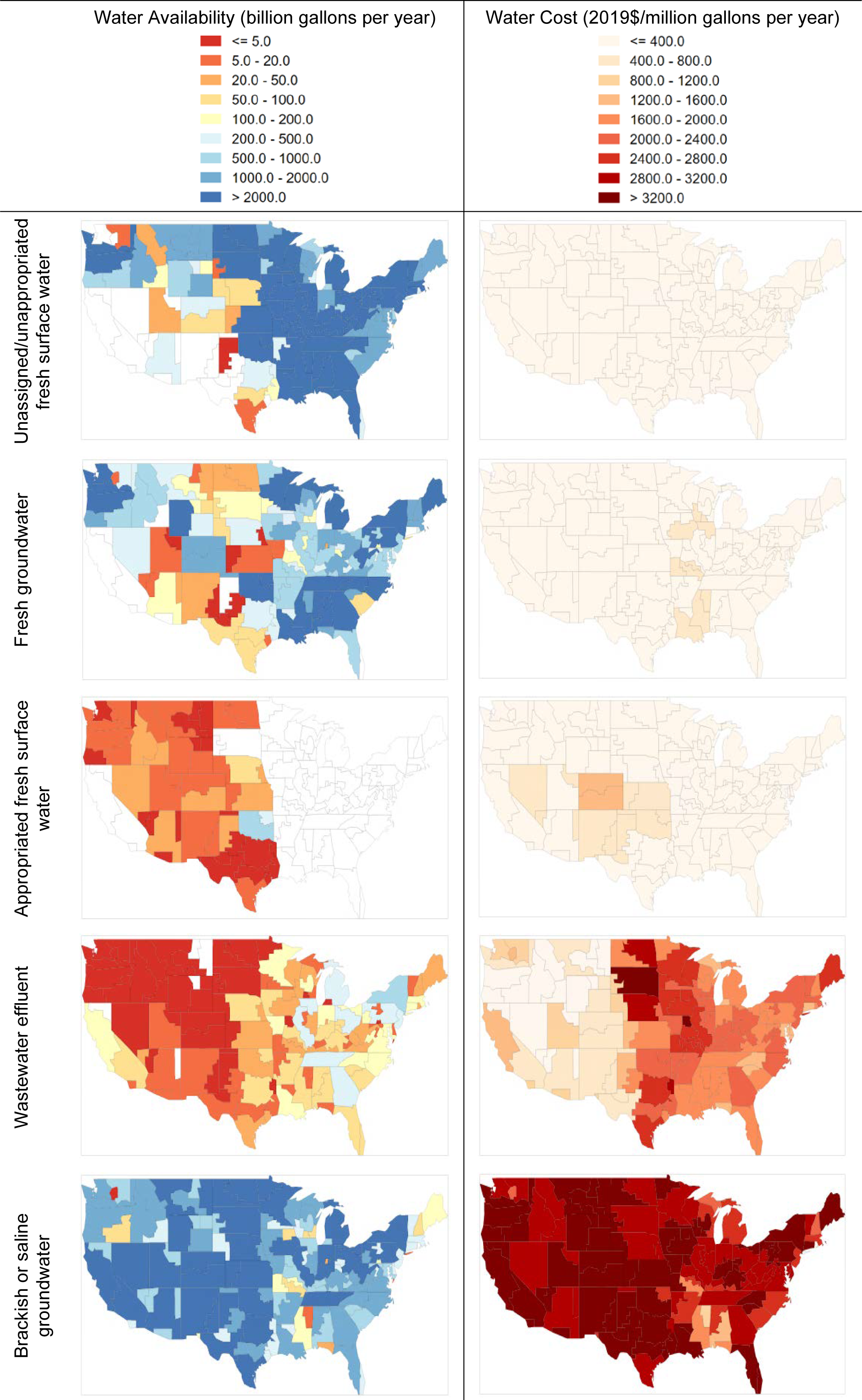
Fig. 62 Water availability and cost for each water type in each ReEDS zone.
Water Constraints
Several model constraints govern the ReEDS power sector water use formulation. Water withdrawal and consumption quantities are tracked for each power technology, cooling technology, water source, power technology vintage, zone, time slice, and year, providing high resolution with which to examine power sector water use. Separately, water access requirements are related explicitly to the capacity available for each power technology, cooling technology, water source, power technology vintage, zone, and year based on either the withdrawal or consumption rate as described in the Water Availability and Cost section. This water access is then limited by the total access available for each water source and region as defined by the water allocation in 2010 and the supply available to post-2010 capacity.
Quantities of water used for each power technology, cooling technology, water source, power technology vintage, and zone are then constrained within each representative day based on an assumed quarterly (winter, spring, summer, fall) allocation of available water access and the relative weight of each quarter in each representative day. Water access must be purchased from the water availability supply curve before water can be used. Hydrology data are used to define the quarterly allocation of unassigned/unappropriated fresh surface water [Macknick et al., 2015], and all other water types are assumed available uniformly throughout the year. Additional resolution for intraannual water allocation or the potential for changes over time requires additional data, but the framework generally allows the capability to incentivize water sources that are more available when electricity demands are higher.
Air Pollution
CO2 and CO2e
ReEDS includes upstream and process emissions of CO2 and CO2e (including CO2, CH4, N2O, and H2). CO2e emission (\(\text{EMIT}(\text{CO}_{2}e)\)) is defined as:
where EMIT(\(p\)) is emission from pollutant \(p\) and GWP(\(p\)) is the global warming potential (GWP) of pollutant \(p\). EMIT(\(p\)) is calculated within the model as the heat rate times the fuel emission rate times the generation. The available options for GWPs in ReEDS are shown in Table 23, taken from the Intergovernmental Panel on Climate Change Sixth Assessment Report [IPCC, 2021].
Pollutant |
AR4-100 |
AR4-20 |
AR5-100 |
AR5-20 |
AR6-100 |
AR6-20 |
|---|---|---|---|---|---|---|
CO2 |
1 |
1 |
1 |
1 |
1 |
1 |
CH4 |
25 |
72 |
34 |
86 |
29.8 |
82.5 |
N2O |
298 |
289 |
298 |
268 |
273 |
273 |
Global warming potentials
The GWP values are located at inputs/emission_constraints/gwp.csv.
Users can add their own GWPs by adding a new column to this file and then specifying their GWP scenario using the GSw_GWP switch in cases.csv or by specifying the GSw_GWP switch following the CH4_{value}/N2O_{value}format directly in cases.csv.
National emissions constraints
The current setting options for CO2/CO2e annual emission caps in ReEDS are as follows:
If setting
GSw_Upstream = 1: CO2/CO2e emissions includes both upstream and process emissions in emission constraints, only process emissions if = 0 (model default). This switch specifies only which type of emission is included in the emission constraints. The emission output files will include both upstream and process emissions regardless of whether a switch is turned on.If setting
GSw_AnnualCap = 0(model default): There are no emission caps for both CO2 and CO2e.If setting
GSw_AnnualCap = 1: Only CO2 emission is capped following emission trajectories defined ininputs/emission_constraints/co2_cap.csv(can be both upstream + process or just process depending onGSw_Upstreamsetting).If setting
GSw_AnnualCap = 2: CO2e emission is capped following emission trajectories defined ininputs/emission_constraints/co2_cap.csv(can be both upstream + process or just combustion depending onGSw_Upstreamsetting).If setting
GSw_AnnualCap = 3: H2 leakage from H2 production, by SMR, SMR-CC and electrolyzer as well as electricity production from H2 combustion plants and fuel cells, is also included in CO2e emissions, which are capped following emission trajectories defined ininputs/emission_constraints/co2_cap.csv.
SO2 and NOx
ReEDS can also output precombustion and combustion SO2 and NOx emissions. There are currently no emission cap trajectories for SO2 in the model, but NOx emission is limited by the Cross-State Air Pollution Rule (CSAPR) detailed in the Policy section below. SO2 and NOx are also included in health damage calculations (see Cost of health damages from air pollution)
Federal, State, and Local Policies
Policies modeled in ReEDS include federal and state-level emission regulations, tax incentives, and portfolio standards. This section primarily focuses on existing policies, but additional frameworks that exist in the model are discussed in Other Policy Capabilities.
Federal and State Emission Standards
EPA’s greenhouse gas emissions regulations
ReEDS represents EPA’s greenhouse gas emissions standards for power plants. For existing coal plants, ReEDS models an emissions rate-based compliance mechanism, enforced at the state level. In 2032 and for every year thereafter, the emissions rate (metric tons CO2 per MWh) of a state’s coal fleet must be less than or equal to the emissions rate of a coal-CCS plant with a 90% capture rate. This enables some unabated coal plants to remain online after 2032 if that state also has coal-CCS plants with high capture rates that stay online and generate, decreasing the average emissions rate. Also starting in 2032, new gas plants must either retrofit with CCS or operate below a 40% capacity factor. Existing gas plants fall outside the scope of this rule.
Cross-state air pollution rule
ReEDS applies the Cross-State Air Pollution Rule using caps on power plant emissions to the states in the eastern half of the United States over which the rules are imposed. From 2017 onward, CSAPR annual emission allowance budgets for NOx are applied at the state level using the Phase 2 caps [EPA, 2008]. The caps are applied only during the ozone season. ReEDS applies a seasonal estimate of these ozone season caps that adjusts for the overlap of ReEDS season definitions and ozone season definitions. States can trade allowance credits within the eligible trading groups but must keep emissions below the required assurance levels.
Sulfur dioxide (SO2) emission limits are not represented in the model because the caps would not be binding in the model except in historical years.
Mercury and Air Toxic Standards
Because compliance with the Mercury and Air Toxic Standards (MATS) has already been largely achieved, we do not represent MATS in the ReEDS model.
California carbon cap
California’s Global Warming Solution Act of 2016 (referred to as Assembly Bill 398 or AB 398) established a program to reduce economywide greenhouse gas emissions to 1990 levels by 2020. In 2016, legislation was passed that codified the 2030 greenhouse gas target to 40% below 1990 levels. In ReEDS, these state carbon caps are modeled as a cap on electricity-system CO2 emissions from generators either located in California or serving load in the state. Direct CO2 emissions from generators located in California count toward the cap. For imported electricity, the model calculates the regional emissions rate (metric tons CO2/MWh) after each solve year and then apply that rate to imports in the next solve year. In scenarios that also have a national carbon cap that reaches zero emissions, the emission intensity of California imports is also set to zero for years when the national carbon cap is zero.
Because California’s greenhouse gas reduction targets are legislated for all economic sectors whereas ReEDS models only the electricity sector, we rely on published economywide modeling results to estimate electric-sector-specific caps that are used in ReEDS. In particular, we apply power sector caps based on the annual California electric sector emissions (from in-state and imported electricity) from California Public Utilities Commission [CPUC, 2018], which provides guidance for a 42 million tCO2 cap by 2030. We enforce that cap from 2030 to 2050. The pre-2030 cap ramps linearly from 60 million tCO2 in 2020 to the 42 million tCO2 in 2030. Note we also model California’s RPS policy.
Delaware carbon cap
In August 2023, Delaware passed House Bill 99, which established a series of emissions goals. EIA reports annual state emissions from which the 2005 baseline was taken. The 2030 target is set as 50% of the 2005 levels and linearly interpolated to reach 0 by 2050. The 2023–2029 are backward-interpolated from the 2030 value.
Regional Greenhouse Gas Initiative
The Regional Greenhouse Gas Initiative (RGGI) cap-and-trade program limits the CO2 emissions for fossil-fuel-fired power plants in 10 states: Connecticut, Delaware, Maine, Maryland, Massachusetts, New Hampshire, New Jersey, New York, Rhode Island, and Vermont.
One RGGI allowance equals the authorization of a regulated fossil fuel power plant 25 MW and greater to emit 1 short ton of CO2. Past and current RGGI allowances can be downloaded from https://www.rggi.org/allowance-tracking/allowance-distribution. The sum for the column “CO2 Allowance or Base Budget” was used (total number of CO2 allowances allocated by each state). This column was used because it best represents the total CO2 amounts that are permitted to be emitted. The “CO2, Allowance Adjusted Budget” column, for example, shows the budgets of each state after the banked allowances have been subtracted from the base budget. Banked allowances are stored CO2 allowances that have accumulated through the previous control periods, which are roughly the previous 4–5 years. Future RGGI allowances (regional scale) through 2030 were provided by RGGI employee Cooper Tamayo. We assume the budget remains constant beyond 2030. We do not model banking of allowances, emissions offsets, or recycling of initiative allowance revenues.
Federal and State Tax Incentives
Federal tax credits for clean electricity and captured carbon
Existing federal tax incentives are included in ReEDS, aligned with the One Big Beautiful Bill Act (OBBBA) passed in the summer of 2025. These include the production tax credit (PTC) and the ITC for several electricity generation technologies, the 45Q credit for capturing and storing carbon, the 45U credits for existing nuclear generation, the 45V credit for producing hydrogen, and the Modified Accelerated Cost Recovery System (MACRS) depreciation schedules.
Four clean electricity production and investment tax credits are represented in ReEDS:
Production Tax Credit (PTC): $26/MWh for 10 years (2022 dollars) plus a bonus credit that starts at $1.3/MWh and increases to $2.6/MWh by 2028 for eligible technologies.
Investment Tax Credit (ITC): 30%, plus a domestic content bonus credit that starts at an additional 2.5% and increases to 5% by 2028 (for totals of 32.5% and 35%, respectively). Energy community bonuses are also applied based on the location of the new build, with an additional 10% bonus for building within an energy community. For ReEDS regions that are only partially covered by energy communities, the 10% bonus is derated by the portion of the region (by land area) that is made up of energy communities.
Captured CO2 Incentive (45Q): $85 per metric ton of CO2 for 12 years for fossil-CCS and bioenergy-CCS and $180 per metric ton of CO2 for 12 years for direct air capture; nominal through 2026 and inflation adjusted after that.
Existing Nuclear Production Tax Credit (45U): This tax credit is $15/MWh (2022 dollars), but it is reduced if the market value of the electricity produced by the generator exceeds $25/MWh. As a simplification, this dynamic calculation was not directly represented in ReEDS. Instead, to represent the effect of this provision, existing nuclear generators are not subject to economic retirement in ReEDS through 2032.
Hydrogen Production Tax Credit (45V): Up to $3/kg of hydrogen produced, based on the life-cycle emissions of hydrogen production, with more emitting generation able to claim lower levels of the tax credit. $3/kg is in $2022 and the credit amount is inflation adjusted in subsequent years. ReEDS assumes the $3/kg credit is sufficient incentive for all hydrogen producers to comply with the mechanisms required to prove the cleanliness of their electricity and therefore allows only generation technologies that qualify for the lowest life-cycle emissions category to contribute.[28]
The tax credit rules allow for bonus credits for both the clean electricity PTC and ITC (but not 45U or 45Q) if a project either meets certain domestic manufacturing requirements or is in an energy community. Projects can obtain both bonus credits if they meet both requirements, which would equate to $5.2/MWh for the PTC and 20% for the ITC. In ReEDS, this is simplified according to the summary above. In practice, there will likely be greater diversity of captured credits among projects. Relatedly, the values above are based on the assumption that all projects will meet the prevailing wage requirements.
Eligible electricity projects can select whether to take the PTC or the ITC. As implemented in ReEDS, however, an a priori analysis was performed to estimate which credit was most likely to be more valuable, and the technology was assigned that credit. The assignments are as follows:
PTC: Land-based wind, utility-scale PV, and biopower
ITC: Offshore wind, CSP, geothermal, hydropower, new nuclear (both conventional and SMR), PSH, distributed PV, and batteries.
PV-battery gets both the PTC and ITC in ReEDS. PTC is applied only to the PV portions of PVB generation, and ITC is applied to the battery component.
As represented in ReEDS, the value of the tax credits is reduced by 10% for non-CCS technologies and 7.5% for CCS technologies, as a simple approximation of the costs of monetizing the tax credits (such as tax equity financing).[29] These cost penalties are not reflected in the values given for each incentive above.
Under OBBBA, solar and wind technologies need to have commenced construction in 2026 or be completed by the end of 2027 to be eligible for tax credits. Projects that meet the commenced construction requirements and come online after 2027 have additional requirements (e.g., foreign entity of concern) they must meet in order to be eligible for the tax credits. Because of the uncertainty about whether post-2027 projects will be eligible for tax credits, ReEDS includes two options to represent incentives: one that allows solar and wind projects coming online through the end of 2030 to receive the tax credits and one that assumes only projects coming online by 2027 will receive the tax credits.
Technologies other than solar and wind can continue to receive the PTC and ITC through 2032, adjusted for under-construction provisions. The 45V tax credits are scheduled to end at the end of 2027 (adjusted for under-construction provisions), and the 45Q and 45U credits are scheduled to end at the end of 2032 (again, adjusted for under construction provisions).
In the dGen model, distributed PV is assumed to take an ITC: the 25D credit for residential, and the Section 48 credit for commercial and industrial. Because the current dGen model runs were created under IRA, for residential projects placed in service through 2032, the ITC is assumed to be 30%, declining to zero for projects placed in service in 2036. For commercial and industrial projects coming online through 2035, the ITC is assumed to be 40%, dropping to zero after that. These representations are simplifications because there can be greater diversity in captured value depending on factors such as ownership type and tax status. IRA includes additional bonus credits (up to 20%) for up to 1.8 GW per year for solar facilities that are placed in service in low-income communities. The dGen model runs used in ReEDS does not have an explicit representation of that additional bonus credit. Instead, 0.9 GW per year of distributed PV was added to the original dGen estimates through 2032. The estimate of 0.9 GW reflects the assumption that some of the projects capturing the bonus credit may not be additional (i.e., they would have occurred anyway even if the bonus credit was not available). The 0.9 GW per year is added in such a way that the spatial distribution of distributed PV remains unchanged.
ReEDS can also be run with the federal tax incentive changes introduced by the One Big Beautiful Bill Act (OBBBA). Under OBBBA, solar and wind projects must either start construction by July 4, 2026 or come online by the end of 2027 to be eligible for the PTC and ITC, and hydrogen projects must start construction by the end of 2027 to be eligible for the hydrogen PTC. The new law also introduces foreign entity of concern (FEOC) restrictions, which can render projects ineligible for tax credits depending on their level of involvement with prohibited foreign entities. ReEDS reflects these provisions through reference and conservative scenarios. The reference scenario updates the safe harbor periods for utility-scale PV, CSP, land-based wind, and offshore wind so that plants must come online by 2029 to be eligible for tax credits. This assumes that all plants starting construction before July 4, 2026 will come online by 2029 while meeting FEOC requirements. The conservative scenario updates the safe harbor periods for these technologies so that plants must come online by 2027 for eligibility. This assumes that FEOC restrictions will prevent most developers from cost-effectively using the tax credit. Both scenarios require hydrogen plants to come online by 2031 to be eligible for the hydrogen PTC, reflecting the notion that developers must start construction by 2027 and taking into the account the standard 4-year safe harbor period. OBBBA also expands eligibility for the energy community bonus to include nuclear plants placed in nuclear energy communities, or metropolitan statistical areas for which at least 0.17 percent of direct employment has been related to nuclear power at any point since 2010.
Tax incentive settings
The incentive scenario (ira, obbba, obbba_conservative, etc.) is controlled by the
incentives_suffixswitchThe tax incentives corresponding to a given scenario are specified in the
inputs/financials/incentives_{incentives_suffix}.csvfile
State Renewable Portfolio Standards
ReEDS models state RPSs, including technology set-asides and renewable energy certificates (RECs) that can count toward RPS compliance. RPS rules are complex and can vary significantly between states. The RPS representation in ReEDS attempts to model the primary impacts of these RPS rules but includes many simplifying assumptions. In addition, in recent years there have been numerous changes to RPS legislation. We periodically update our representation to capture the recent changes to the legislation; however, the numerous and frequent changes to state laws create challenges to having a precise representation of all RPS legislation.
RPS targets—along with many other data that we use to represent nuanced RPS rules—are based on data compiled by Lawrence Berkeley National Laboratory, which takes into account the in-state REC multiplier incentives and load adjustments (e.g., sales-weighted RPS targets considering different load-serving entities subject to compliance, such as investor-owned utilities, municipal utilities, and cooperatives) [Barbose, 2024, LBNL, 2025]. Solar includes UPV and rooftop PV, wind includes both land-based and offshore technologies, and distributed generation (DG) includes rooftop PV and ground-mounted PV systems located within the distribution network.[30] ReEDS also models alternative compliance payments for unmet RPS requirement for both main RPS targets and solar/wind set-asides as is consistent with the available data.
RPS input data
RPS targets and technology set-asides for 2010-2050 can be found in /inputs/state_policies/rps_fraction.csv.
Technology eligibility for state RPS requirements is modeled for each state.[30] For instance, California’s RPS does not allow in-state rooftop solar technologies to contribute toward its RPS. In addition, every state has specific rules regarding hydropower generation’s eligibility toward contributing RECs, which are usually based on each unit’s vintage and size (e.g., small hydropower with specific capacity cutoffs are eligible in some states). ReEDS models these as allowable generation fractions from Barbose 2024, which is imposed on each state’s total hydropower generation, limiting the amount of hydropower RECs that each state could produce.
Except for California, ReEDS enforces an upper limit on the total RECs (both bundled and unbundled) that can be imported for that state’s RPS compliance.
For California alone, because of its unique out-of-state rules, ReEDS enforces two upper limits: one on the total unbundled REC imports and the other on the total bundled REC imports.
There are myriad possibilities of interstate REC transactions, in terms of both which two states can transact and the quantity of those transactions.
To constrain the solution space of ReEDS to credible values, the interstate REC trading modeling is based on historical observations [Holt, 2016] and captured by inputs/state_policies/rectable.csv.
The out-of-state total REC import percentages for each state are limited to those observed in 2012–2013 [Heeter, 2015] with additional updates made over the years based on state input and observed trading behavior.
To prevent laundering of credits through two states that are not allowed to trade but have a common trading partner, ReEDS includes a requirement that a state may not export more credits than it can produce. If a state is using alternative compliance payments to meet its RPS or clean energy standard (CES) requirement, that state is further limited in its ability to export credits.
Several states have implemented policies directed at offshore wind. To represent these actions in ReEDS, we prescribe a floor to offshore wind capacity based on known projects and policy mandates. Specifically, we include offshore wind capacity that meets at least one of three criteria: current operating capacity, projects in active solicitation processes, and statutory policy requirements. The projects are based on tracking conducted for the NREL Offshore Wind Technologies Market Report, and state totals are shown in Table 24.[31] The model allows economic deployment of offshore wind capacity beyond these levels. All policy-mandated offshore wind capacity is assumed to be rebuilt if retiring the capacity would bring the total below the mandated limit.
Finally, voluntary renewable energy credits are also represented in ReEDS. Only renewable energy technologies are allowed to supply voluntary RECs, and Canadian imports are not allowed. The voluntary REC requirement is based on the observed amount of voluntary RECs from [Heeter et al., 2021], and the requirement is assumed to grow by the smallest amount that has been observed year-over-year (0.1624% in absolute terms). The voluntary requirement includes an alternative compliance payment of $10/MWh (in 2004$).
State |
2020 |
2030 |
2040 |
2050 |
|---|---|---|---|---|
CA |
— |
60 |
7,602 |
7,602 |
CT |
- |
2,000 |
2,000 |
2,000 |
MA |
— |
3,916 |
5,600 |
5,600 |
MD |
— |
2,675 |
8,500 |
8,500 |
ME |
— |
156 |
3,000 |
3,000 |
NJ |
— |
1,510 |
11,000 |
11,000 |
NY |
— |
3,801 |
9,000 |
9,000 |
RI |
30 |
1,430 |
1,430 |
1,430 |
VA |
12 |
3,230 |
5,200 |
5,200 |
Total |
42 |
18,778 |
53,332 |
53,332 |
Clean Energy Standards
As of November 2024, 16 states had clean energy standards (see Table 25). CES values are effective values[32] and are taken from [Barbose, 2024]. These CESs are in effect generalized versions of RPSs; their model representations are very similar with technology eligibility being the primary difference.
CES input data
The annual compliance for states with a CES policy can be found in inputs/state_policies/ces_fraction.csv.
For all but one of the CES policies (Massachusetts), we assume all zero-carbon-emitting sources (on a direct emissions basis) can contribute to the CES requirement. This includes all renewable energy technologies (including hydropower and distributed PV), nuclear power, and imports from Canada.[33] The modeled CES policies set a floor on electricity generated from clean energy technologies but does not cap generation from conventional sources. As a result, in the model representation, a state can continue to generate from existing fossil plants if the amount of clean energy generation exceeds the requirement (even if the requirement approaches 100% of sales). Most of the CES policies are assumed to start in 2030 and ramp to their final targets by 2040 or 2050.[34] For other aspects of the CES model representation, we use the same assumptions as the corresponding state RPS. These include assumptions about credit trading and variations in load-serving entity requirements. In the case of Virginia, fossil plants are required to retire according to the schedule indicated in the clean energy policy. Based on discussions with stakeholders, fossil plants in Illinois and New York are also required to retire once the policy reaches the nominal 100% target.[35]
State |
2020 |
2025 |
2030 |
2035 |
2040 |
2045 |
2050 |
|---|---|---|---|---|---|---|---|
CA |
0% |
0% |
57% |
86% |
90% |
95% |
95% |
CO |
0% |
0% |
47% |
48% |
48% |
48% |
56% |
CT |
0% |
0% |
43% |
71% |
99% |
99% |
99% |
IL |
0% |
0% |
35% |
48% |
62% |
75% |
89% |
MA |
23% |
55% |
64% |
72% |
80% |
88% |
96% |
ME |
0% |
0% |
76% |
81% |
86% |
90% |
95% |
MI |
0% |
42% |
61% |
72% |
80% |
100% |
100% |
MN |
0% |
0% |
74% |
90% |
100% |
100% |
100% |
NC |
0% |
0% |
40% |
50% |
60% |
70% |
80% |
NE |
0% |
0% |
0% |
0% |
10% |
50% |
100% |
NM |
0% |
0% |
0% |
0% |
68% |
83% |
90% |
NV |
0% |
0% |
43% |
56% |
68% |
80% |
90% |
NY |
0% |
0% |
70% |
70% |
100% |
100% |
100% |
OR |
0% |
20% |
55% |
62% |
68% |
68% |
68% |
VA |
0% |
36% |
44% |
54% |
66% |
78% |
80% |
WA |
13% |
56% |
100% |
100% |
100% |
100% |
100% |
Storage Mandates
Ten state storage mandates are represented in ReEDS and are summarized in Table 26. The mandates are required to be met with battery storage, and any duration of storage qualifies.
State |
2020 |
2030 |
2050 |
|---|---|---|---|
CA |
1,325 |
2,325 |
2,325 |
MA |
50 |
50 |
50 |
MD |
2,102 |
3,000 |
|
MI |
2,500 |
2,500 |
|
NJ |
600 |
2,000 |
2,000 |
NV |
1,000 |
1,000 |
|
NY |
500 |
3,000 |
3,000 |
OR |
2.5 |
2.5 |
2.5 |
RI |
195 |
195 |
|
VA |
42.7 |
1,350 |
3,100 |
Nuclear Power Plant Policies
There are four states that have enacted policies that provide compensation or other assistance for in-state nuclear power plants: Connecticut, Illinois, New Jersey, and New York. For these states, the nuclear power plants are not allowed to retire until after the policy expires, unless the power plant already has an announced retirement date. The policy end dates are taken from EIA 2019.
In addition, there are several states that do not allow new nuclear power. These states include California, Connecticut, Illinois, Maine, Massachusetts, Minnesota, New Jersey, New York (Long Island only), Oregon, Rhode Island, and Vermont.
Other Policy Capabilities
In addition to the existing policies described above, ReEDS also includes several optional policy implementations that are useful for exploring alternative futures or the impact of existing policies. These additional policy frameworks include:
National Clean Energy Standard: This framework allows the user to specify which technologies count as “clean energy” and enforce a minimum limit for the generation fraction of these clean energy technologies.
National Renewable Portfolio Standard: This standard enforces a national RPS, with the RPS trajectory defined by the user.
Carbon Cap-and-Trade: This feature allows the user to specify national or subnational carbon cap-and-trade policies, including options to represent trading limitations and banking and borrowing of allowances.
Carbon Tax: This feature implements a user-specified carbon tax on burner-tip emissions from the power sector.
National Emissions Limit: This framework limits the total national emissions according to user-specified values. The limit is often referred to as a carbon cap or CO2 cap.
National CO2 cap trajectories
Users can specify these CO2 cap trajectories and/or add their own in inputs/emission_constraints/co2_cap.csv.
National emissions limit is turned off by default but can be turned on in cases.csv by using GSw_AnnualCap.
The cap is applied on a net basis, so negative emission technologies can offset power plant emissions.
Users can restrict negative emissions technologies to offset emissions only from fossil CCS plants by setting GSw_NoFossilOffsetCDR in cases.csv to 1 (the default value is 0).
Subnational Emissions Limit: For subnational ReEDS runs with the CO2 emissions limit turned on and CO2 cap specified, the subnational emissions limit is automatically scaled down from the national emissions limit above to the subnational region that the user defines, based on eGRID’s 2022 county-level CO2 emissions.
Alternative ITC and PTC Schedules: In addition to the ITC and PTC schedules described in Federal and State Tax Incentives, the ITC and PTC can be modified to apply for any number of years and to any technology.
Alternative Financing Measures: Policy-related financing impacts such as MACRS or the under-construction provisions for the ITC and PTC can be modified as specified by the user.
Capital Financing, System Costs, and Economic Metrics
Financing of Capital Stock
The financing assumptions used in ReEDS are taken directly from the 2024 ATB spreadsheet [NREL, 2024], using the “Market Factor Financials” and the 30-year capital recovery period options. The ATB has technology-specific and time-varying financing parameters, including interest rate, rate of return on equity, debt fraction, and tax rate. Other elements of the ATB included in ReEDS include construction schedules, MACRS depreciation schedules, and inflation rates. These values are further defined and explained in the ATB, with additional explanation of our financing implementation detailed in the (6) of the appendix.
Cost calculations within the model are done assuming a 30-year economic lifetime for all generation assets (transmission lines and AC/DC converters have a 40-year economic lifetime). Technologies with a physical lifetime shorter than the economic lifetime have a penalty applied to reflect the need for a replacement before the end of the economic life.
Electric Sector Costs
Two systemwide cost metrics are calculated from each ReEDS run: a present value of direct electric sector system costs and electricity price. These cost calculations are not part of the ReEDS optimization process; they are calculated after the ReEDS optimizations have been conducted. ReEDS also includes a postprocessing option for estimating retail rates and for estimating the health costs of air pollution, described further below.
Present value of direct electric sector cost
The present value system cost metric accounts for capital and operating expenditures incurred over the entire study horizon for all technology types considered, including generation, transmission, and storage. The cost in each future year is discounted by a social discount rate, by default set to 2% [OMB, 2023]. The social discount rate is not to be confused with the investment discount rate used in the optimization for investment decisions; the investment discount rate is selected to represent private-sector investment decisions for electric system infrastructure, and it approximates the expected market rate of return of investors. Capital costs incurred before the start of the specified economic horizon are annualized and included in the system cost metric. Details about how the system costs are calculated in ReEDS can be found in the Calculating Present Value of Direct Electric Sector Cost section of the appendix.
Electricity price
ReEDS calculates “competitive” electricity prices at different regional aggregation levels [EIA, 2017, Murphy and Smeers, 2005, Ventosa et al., 2005]. This calculation takes advantage of the linear programming formulation of the model. Specifically, the marginal price on a model constraint represents how much the objective function would change given a change in the right side of the constraint. Each constraint can be viewed as a market with a marginal price and quantity. At optimality, the total revenue (i.e., the product of price and quantity) across all constraints equals the objective function value. The constraints within ReEDS are written so the marginal values from the load constraints can be used as a proxy for the competitive electricity price. The load constraints are linked to the supply-demand balance constraints, capacity constraints, operating reserve constraints, and others through load variables. Taking the marginal value from the load balance constraint, we can find the marginal value of an additional unit of load (e.g., MWh) to the system, accounting for other requirements. Specifically, the reported competitive prices in ReEDS capture five categories of requirements: energy, capacity, operating reserves, and state-level and national-level RPS requirements (see Table 27). The competitive prices can be reported at different regional aggregation levels, scaled by requirement quantities. Details about how these prices are calculated in ReEDS can be found in the Marginal Electricity Prices section of the appendix.
Constraint Category |
Grid Service (s) |
Region (r) |
Time (h) |
Units - Price |
Units - Quantity |
|---|---|---|---|---|---|
Operation |
Energy |
Zone |
Time slice |
$/MWh |
MWh |
Operation |
Flexibility reserve |
Zone |
Time slice |
$/MWh |
MWh |
Operation |
Regulation reserve |
Zone |
Time slice |
$/MWh |
MWh |
Operation |
Spinning reserve |
Zone |
Time slice |
$/MWh |
MWh |
Resource Adequacy |
Capacity |
Zone |
Season |
$/kW-yr |
kW |
Policy |
State RPS |
State |
Annual |
$/MWh |
MWh |
Policy |
National RPS |
National |
Annual |
$/MWh |
MWh |
Policy |
CO2 cap |
National |
Annual |
$/metric ton |
metric ton |
Policy |
RGGI CO2 cap |
Regional |
Annual |
$/metric ton |
metric ton |
Policy |
SB32 CO2 cap |
Regional |
Annual |
$/metric ton |
metric ton |
Besides “competitive electricity prices,” ReEDS also calculates the average cost of electricity at the national, zonal, or state level by taking the annualized total costs of building and operating the system in a specific geographic area and dividing that by the electricity load in that area. Annualized costs for existing (i.e., pre-2010) power plants are also considered given plants’ initial investment costs and the build year. Zonal average electricity prices also consider the impact of energy and capacity trading. These prices reflect the average costs to serve the load in certain areas. Detailed calculation equations can be found in the Average Electricity Prices section of the appendix.
Retail rates
ReEDS estimates average retail electricity rates using the method described by [Brown et al., 2022]. This retail rate method is a separate module run after a ReEDS run has been completed. It uses a detailed bottom-up accounting method for projecting retail rates based on the ReEDS buildout and operation. It uses an accounting framework most aligned with an investor-owned utility and accounts for depreciation, taxes, and the breakdown between operating and capitalized (rate-based) expenses. Distribution, administration, and intraregional transmission costs are projected forward based on empirical trends from 2010 to 2019. For more details on the method, see [Brown et al., 2022].
The retail rate method has since been expanded to handle negative emission technology cost allocation. Because the retail rate method reports state-level average retail rates, if one state builds a negative emission technology such as DAC or BECCS, that state will incur the costs even though the emissions offset by that unit are likely to be from another state. The retail rate method allocates the cost of the negative emission technology to the states with CO2 emissions, weighted by the amount of CO2 emissions.
Cost of health damages from air pollution
In addition to direct system costs, ReEDS also includes a postprocessing step for estimating health damages associated with air pollution. Currently this focuses on mortality from long-term exposure to fine particulate matter (PM2.5) from fossil fuel combustion in the electric sector. Previous work has found that accounting for mortality results in the largest component of monetized benefits [EPA (U.S. Environmental Protection Agency), 1999, NRC (National Research Council), 2010] and that PM2.5 exposure is the driver of 90%–95% of all mortalities related to air pollution [Tessum et al., 2017, Tschofen et al., 2019].
To estimate health damages, ReEDS relies on estimates of the mortality risk per tonne of emissions from three reduced complexity air quality models (AP2, EASIUR, and InMAP) [Center for Air, Climate, and Energy Solutions, 2025]. Each of these models estimates PM2.5 formation associated with emissions of precursor pollutants (NOx and SO2). To generate annualized premature mortality, each model applies a concentration response function from one of two studies linking exposure to PM2.5 to increased mortality risk. These two studies, referred to as the American Cancer Society Study and Harvard Six-Cities Study, provide estimates of the relationship between pollution exposure and premature mortality [Gilmore et al., 2019]. The result is an estimate of the mortality risk per tonne of pollutant emitted in each U.S. county. This marginal damage estimate can be aggregated to zonal resolution and multiplied by total emissions to estimate total mortality.
As a final step, annual premature deaths from air pollution can be translated into a monetary value by applying a value of a statistical life. For this, ReEDS relies on EPA’s estimate of $7.4 million in $2006 [EPA (U.S. Environmental Protection Agency), 2014] inflated to a present-day dollar value ($11.5 million in $2024). These costs can then be translated into costs per unit of generation and cumulative (discounted) cost over the study period.
The approach described here focuses on direct emissions from the electric power sector and thus does not capture estimates from other sectors (such as transportation, buildings, and industry) or upstream emissions (such as from fossil fuel extraction or power plant manufacturing). It also does not quantify any social costs of climate change from CO2 or other greenhouse gas emissions.
Modeled Economic Metrics
ReEDS calculates multiple economic metrics for analyzing investment decisions in the model, including the following:
Levelized cost of energy (LCOE)
Technology value
Net value of energy (NVOE)
Net value of capacity (NVOC)
System profitability.
These metrics are described in detail below.
Levelized cost of energy
LCOE measures the unit cost of electricity of a specific technology, which is normally calculated as lifetime costs divided by energy production. Specifically, the LCOE is calculated as follows [NREL, 2019]:
where FCR is the fixed charge rate; CAPEX is the capital expenditures; FOM is the fixed operations and maintenance costs; CF is the capacity factor; 8760 is the number of hours in a year; VOM is variable operations and maintenance costs; and FUEL is fuel costs (if applicable).
In each model year, ReEDS reports the LCOE for all technology options considering different variations in tax credit treatments and capacity factor assumptions. ReEDS also calculates the LCOE for technologies that are built in this model year using the generation from these technologies.
Technology value
ReEDS reports the value that generators receive from providing grid services. Value is calculated as the product of service prices and service provision quantities. For example, the value of a generator that comes from providing energy service to meet planning reserve margin requirement is calculated as the price of capacity multiplied by the amount of firm capacity the generator can provide. The reported revenues capture energy, capacity, operating reserve, and state-level and national RPS requirements. Revenues can be normalized either by the amount of generation or by the amount of installed capacity.
Revenues are closely related to, but are different from, the electricity price and service requirement quantity parameters. Revenues consider the provision of different services from a certain generator in a region, whereas service requirement quantities calculate the demand of different services in a region. The sum of revenues from all generating technologies in a specific region does not necessarily equal the sum of products of all service prices and corresponding service requirements.
Net value
ReEDS reports different economic viability metrics that consider both costs and values of generating technologies to fully evaluate the economic competitiveness of a certain technology and to provide intuitive explanations about investment decisions in the model. “Values” of a generator reflect the potential economic benefit from displacing or avoiding the cost of providing the services from other (marginal) assets, whereas “costs” aggregate all different sources of costs needed to build and operate a power plant to provide services. We define “net value” as the difference between values and costs. Net value is related to a concept in linear programming called “reduced cost.” Mills and Wiser 2012 describe reduced cost in the context of electricity system modeling.
We report three types of such metrics to assess the economic viability of generators: net value of energy, net value of capacity, and system profitability metrics (Table 28). These metrics are reported both for new investments in a certain model year and for existing generators that have been built.
Metric |
Conceptual Expression (typical units) |
|---|---|
Net value of energy (NVOE) |
(Value – Cost)/Energy ($/MWh) |
Net value of capacity (NVOC) |
(Value – Cost)/Capacity ($/kW-yr) |
System profitability |
(Value/Cost) (unitless) |
NVOE measures the unit profit of a specific technology, calculated as the difference between generator revenue and costs, then normalized by the energy production. The typical unit is dollars per megawatt-hour ($/MWh). Similarly, NVOC measures the unit profit of a specific technology, calculated as the difference between generator revenue and costs, then normalized by the installed capacity. The typical unit is dollars per megawatt ($/MW).
Both of these metrics are normalized metrics; because the denominators vary broadly for different generator types, they may not reflect the competitiveness of technologies consistently. Therefore, we report a third type of economic viability metric—system profitability metrics—which are essentially unitless functions of the ratio between values and costs. Examples include profitability index (value/cost) and return on investment (value/cost minus one). We report both metrics in ReEDS, acknowledging there are other formats of system profitability metrics.
These economic viability metrics help explain investment decisions in the model. Specifically, for all types of new investment in a certain model year, the model considers all the costs to build and operate a certain technology as costs and the contribution of the technology to all binding constraints as values (i.e., service provision). Typical value sources are discussed above in Technology Value. In calculations of economic viability metrics, however, other types of “values” are included to fully reflect model decisions. For example, an increase in ancillary service requirements because of increased wind generation fraction is counted as a negative value stream for wind, and it is included in the metrics calculation here. Therefore, these metrics fully reflect all the model constraints related to the investment decision.
Uncertainty Modeling Capabilities
Monte Carlo Sampling
ReEDS includes a Monte Carlo Sampling (MCS) module designed to help quantify how uncertainty in key model inputs affects capacity expansion outcomes. This module supports regionalized sampling, grouped or independent treatment of input switches, and multiple distribution types. For each run, the module draws input values from user-defined probability distributions, writes the corresponding input files, and executes a set of ReEDS runs. Results can then be aggregated to evaluate ranges, quantiles, and other metrics derived from model outputs.
For step-by-step instructions on running ReEDS with MCS, required switches, and how to define custom distribution groups, see the Monte Carlo Sampling (MCS) section of the User Guide.
Modeling to Generate Alternatives
ReEDS includes a simple implementation of “Modeling to Generate Alternatives” (MGA) [Neumann and Brown, 2021]. The high-level procedure when applying MGA as implemented in ReEDS is:
Solve the model minimizing the normal system-cost objective function
Define a cost envelope around the optimized objective function value (typically in the range of 1%)
Rerun the model with a different objective function (thus exploring “alternatives” to the single optimal solution, helping characterize the steepness or shallowness of the solution space)
The available options for the secondary objective are:
Min/max the capacity of a given tech group (e.g., fossil, upv, wind, battery, nuclear, etc.)
Min/max the total MW capacity of interzonal transmission
Min/max the MWh of stress period flows between NERC regions (“RA sharing”)
Min/max direct CO2 emissions
Relevant model switches are described in the Modeling to Generate Alternatives (MGA) section of the User Guide.
Model Linkages
ReEDS-PCM
The ReEDS reduced-form dispatch and variable renewable parameterization aims to represent enough operational detail for realistic capacity expansion decisions, but the model cannot explicitly represent detailed power system operations. To enable more detailed study of system operations, NREL has developed a translation framework R2X to implement a ReEDS capacity expansion solution for any solve year in production cost models (PCMs). R2X supports translations to mainstream PCMs: Sienna and PLEXOS. See here for the latest ReEDS model compatibility with R2X.
Sienna is an open-source NREL modeling tool for scientific energy system analysis.
As part of its core capabilities, Sienna\Ops supports the simulation of system scheduling—including unit commitment and economic dispatch, automatic generation control, and nonlinear optimal power flow—along with sequential problem specifications to enable production cost modeling techniques.
NREL has used Sienna in several analyses such as Puerto Rico 100 and the National Transmission Planning Study
where it was used as the PCM tool for transmission planning and operational analysis for future scenarios [DOE, 2024, Murali Baggu et al., 2024].
PLEXOS is a commercial PCM tool capable of representing individual generating units and transmission nodes for least-cost dispatch optimization at hourly or subhourly time resolution. It can incorporate unit-commitment decisions and detailed operating constraints (e.g., ramp rates, minimum runtime) to simulate realistic power system operations. NREL has used PLEXOS in several analyses such as the Western Wind and Solar Renewable Integration Study and the Eastern Renewable Grid Integration Study [Bloom et al., 2016, Lew et al., 2013].
The ReEDS-PCM linkage involves several transformations to the ReEDS solution to prepare it for use in the PCM. These transformations include disaggregating the ReEDS solution and adding the necessary parameters for PCM. To maintain consistency, the linkage preserves the spatial resolution of ReEDS (zone or county) and operates the PCM as a zonal model that matches ReEDS zones (or county) with a simplified transmission interface between them. The PCM translation uses ReEDS transmission line capacity, whereas reactance and resistance are derived from ReEDS transmission properties to represent the aggregated transmission system. For generating capacity, ReEDS aggregate capacity is converted to individual units in the PCM using characteristic unit sizes for each technology. Where possible and reasonable, ReEDS cost and performance parameters are used, although these values can be improved if more data are available. If a parameter is missing or inconsistently used in ReEDS because of structural differences between the models, the default translation uses average values across the WECC for the equivalent technologies in ReEDS.[36]
Once the ReEDS solution is converted to a PCM, one can simulate hourly dispatch over a full year and compare results with ReEDS outcomes. A consistent solution builds confidence in the effectiveness of ReEDS capacity expansion decisions, whereas inconsistencies and reliability concerns such as load shedding indicate the need for improving capacity expansion model structures. Additional details are available in [Frew et al., 2019].
ReEDS-Cambium
Leveraging the capabilities of the ReEDS-PCM linkage, a third model—Cambium—has been developed. Cambium draws from ReEDS and PLEXOS model solutions to assemble a structured database of hourly cost and operational data for modeled futures of the U.S. electric sector. In addition to directly reporting some metrics from both ReEDS and PLEXOS (e.g., capacity buildouts from ReEDS and generation by technology from PLEXOS), Cambium postprocesses the outputs from both models to develop new metrics that are designed to be useful for long-term decision making, such as a long-run marginal emission rate.[37]
Datasets derived through Cambium can be viewed and downloaded at https://cambium.nrel.gov/. The documentation for Cambium contains descriptions of the metrics reported in the databases and the methods for calculating those metrics [Gagnon et al., 2023].
ReEDS-reV
The ReEDS supply curve for renewable technologies, including land-based wind, CSP, utility-scale PV, and geothermal are produced by reV.
The ReEDS-reV linkage allows regional ReEDS investment decisions to be mapped backed to individual reV supply curve sites.
Site-specific supply curve data from reV are binned for the ReEDS supply curve by default into 5–40 bins depending on the resource type (see numbins_{technology} in cases.csv).
By tracking the timing and investment decisions within each of these bins, the ReEDS-reV linkage maps regional capacity back to the individual sites from which the bins were derived.
The resulting siting data are used to further the understanding of the ReEDS capacity expansion decisions and identify areas for improvement for resource siting in reV.
The ReEDS-reV linkage is a key component in the translation of ReEDS capacity expansion results to a nodal production cost modeling database.
References
Form EIA-860 detailed data with previous form data (EIA-860A/860B). 2018. URL: https://www.eia.gov/electricity/data/eia860/ (visited on 2020-12-30).
U.S. Energy Information Administration (EIA). Form EIA-923 detailed data with previous form data (EIA-906/920). 2024. URL: https://www.eia.gov/electricity/data/eia923/index.php (visited on 2024-09-26).
Abdulrahman Alassi, Santiago Bañales, Omar Ellabban, Grain Adam, and Callum MacIver. HVDC Transmission: Technology Review, Market Trends and Future Outlook. Renewable and Sustainable Energy Reviews, 112:530–554, September 2019. URL: https://linkinghub.elsevier.com/retrieve/pii/S1364032119302837 (visited on 2024-02-05), doi:10.1016/j.rser.2019.04.062.
Vipin Arora. Estimates of the price elasticities of natural gas supply and demand in the United States. Technical Report MPRA Paper No. 54232, U.S. Energy Information Administration, 2014. URL: http://mpra.ub.uni-muenchen.de/54232/ (visited on 2015-06-30).
Chad R. Augustine, Jonathan L. Ho, and Nathan J. Blair. GeoVision Analysis Supporting Task Force Report: Electric Sector Potential to Penetration. Technical Report NREL/TP-6A20-71833, National Renewable Energy Laboratory, Golden, CO, May 2019. URL: https://www.nrel.gov/docs/fy19osti/71833.pdf (visited on 2020-02-03), doi:10.2172/1524768.
R. L. Bain, W. A. Amos, M. Downing, and R. L. Perlack. Biopower Technical Assessment: State of the Industry and Technology. Technical Report NREL/TP-510-33123, National Renewable Energy Laboratory, Golden, CO, 2003. URL: https://www.nrel.gov/docs/fy03osti/33123.pdf.
Galen Barbose. U.S. State Renewables Portfolio & Clean Electricity Standards: 2024 Status Update. Technical Report, Lawrence Berkeley National Laboratory, Berkeley, CA, 2024. URL: https://live-lbl-eta-publications.pantheonsite.io/sites/default/files/lbnl_rps_ces_status_report_2024_edition.pdf (visited on 2024-01-30).
Philipp Beiter and Tyler Stehly. A Spatial-Economic Cost-Reduction Pathway Analysis for U.S. Offshore Wind Energy Development from 2015-2030. Technical Report NREL/PR-6A20-67204, National Renewable Energy Laboratory, Golden, CO, October 2016. URL: https://www.osti.gov/biblio/1330939-spatial-economic-cost-reduction-pathway-analysis-offshore-wind-energy-development-from (visited on 2018-12-12).
Mark A. Bernstein and James M. Griffin. Regional differences in the price-elasticity of demand for energy. Technical Report NREL/SR-620-39512, National Renewable Energy Laboratory, Golden, CO, 2006. URL: http://www.nrel.gov/docs/fy06osti/39512.pdf (visited on 2015-06-30).
J. Bistline, A. Sowder, S. Bragg-Sitton, B. Dixon, Wesley Cole, Jonathan Ho, Caitlin Murphy, A. Kwon, L. Martin, C. Namovicz, and E. Eschmann. Nuclear Energy in Long-Term System Models: A Multi-Model Perspective. Technical Report 3002023697, Electric Power Research Institute, Palo Alto, CA, April 2022. URL: https://www.osti.gov/servlets/purl/1878753 (visited on 2023-01-23), doi:10.2172/1878753.
Nate Blair, Chad Augustine, Wesley Cole, Paul Denholm, Will Frazier, Madeline Geocaris, Jennie Jorgenson, Kevin McCabe, Kara Podkaminer, Ashreeta Prasanna, and Ben Sigrin. Storage Futures Study: Key Learnings for the Coming Decades. Technical Report NREL/TP-7A40-81779, National Renewable Energy Laboratory, Golden, CO, April 2022. URL: https://www.nrel.gov/docs/fy22osti/81779.pdf, doi:10.2172/1863547.
Nate Blair, Thomas Jenkin, James Milford, Walter Short, Patrick Sullivan, David Evans, Elliot Lieberman, Gary Goldstein, Evelyn Wright, Kamala R. Jayaraman, Boddu Venkatesh, Gary Kleiman, Christopher Namovicz, Bob Smith, Karen Palmer, Ryan Wiser, and Frances Wood. Renewable Energy and Efficiency Modeling Analysis Partnership: An Analysis of How Different Energy Models Addressed a Common High Renewable Energy Penetration Scenario in 2025. Technical Report NREL/TP-6A2-45656, National Renewable Energy Laboratory, Golden, CO, 2009. URL: http://escholarship.org/uc/item/9pv3r5fk.pdf (visited on 2015-03-25).
Aaron Bloom, Aaron Townsend, David Palchak, Joshua Novacheck, Jack King, Clayton Barrows, Eduardo Ibanez, Matthew O'Connell, Gary Jordan, Billy Roberts, Caroline Draxl, and Kenny Gruchalla. Eastern Renewable Generation Integration Study. Technical Report NREL/TP-6A20-64472, National Renewable Energy Laboratory, Golden, CO, August 2016. URL: https://www.osti.gov/biblio/1318192/ (visited on 2018-10-25), doi:10.2172/1318192.
Gregory Brinkman, Dominique Bain, Grant Buster, Caroline Draxl, Paritosh Das, Jonathan Ho, Eduardo Ibanez, Ryan Jones, Sam Koebrich, Sinnott Murphy, Vinayak Narwade, Joshua Novacheck, Avi Purkayastha, Michael Rossol, Ben Sigrin, Gord Stephen, and Jiazi Zhang. The North American Renewable Integration Study (NARIS): A U.S. Perspective. Technical Report, NREL, 2021. URL: https://www.nrel.gov/docs/fy21osti/79224.pdf.
Gregory Brinkman, Mike Bannister, Sophie Bredenkamp, Lanaia Carveth, Dave Corbus, Rebecca Green, Luke Lavin, Anthony Lopez, Melinda Marquis, Joseph Mowers, Matthew Mowers, Leonardo Rese, Billy Roberts, Amy Rose, Shahil Shah, Pranav Sharma, Hongfei Sun, Bin Wang, Bharat Vyakaranam, Zhenyu Huang, Kevin Harris, Chuan Qin, Nader Samaan, Marcelo Elizondo, Tony Nguyen, Quan Nguyen, Kishan P Guddanti, and Patrick Royer. Atlantic Offshore Wind Transmission Study. Technical Report, U.S. Department of Energy, March 2024. URL: https://www.nrel.gov/wind/atlantic-offshore-wind-transmission-study.html.
Maxwell Brown, Wesley Cole, Kelly Eurek, Jon Becker, Dave Bielen, Ilya Chernyakhovskiy, Stuart Cohen, Will Frazier, Pieter J. Gagnon, Nathaniel Gates, Daniel Greer, Sai Sameera Gudladona, Jonathan Ho, Paige Jadun, Katherine Lamb, Trieu Mai, Matthew Mowers, Caitlin Murphy, Amy Rose, Anna Schleifer, Daniel Steinberg, Yinong Sun, Nina Vincent, Ella Zhou, and Matthew Zwerling. Regional Energy Deployment System (ReEDS) Model Documentation: Version 2019. Technical Report NREL/TP-6A20-74111, National Renewable Energy Laboratory, Golden, CO, March 2020. URL: https://www.nrel.gov/docs/fy20osti/74111.pdf (visited on 2019-05-15), doi:10.2172/1505935.
Patrick R. Brown, Clayton P. Barrows, Jarrad G. Wright, Gregory L. Brinkman, Sourabh Dalvi, Jiazi Zhang, and Trieu Mai. A general method for estimating zonal transmission interface limits from nodal network data. August 2023. URL: http://arxiv.org/abs/2308.03612 (visited on 2023-09-26), arXiv:2308.03612.
Patrick R. Brown, Wesley J. Cole, and Trieu Mai. An interregional optimization approach for time series aggregation in continent-scale electricity system models. Energy, pages 135830, April 2025. URL: https://linkinghub.elsevier.com/retrieve/pii/S0360544225014720 (visited on 2025-04-08), doi:10.1016/j.energy.2025.135830.
Patrick R. Brown, Pieter J. Gagnon, J. Sean Corcoran, and Wesley J. Cole. Retail Rate Projections for Long-Term Electricity System Models. Technical Report NREL/TP-6A20-78224, National Renewable Energy Laboratory, Golden, CO, January 2022. URL: https://www.nrel.gov/docs/fy22osti/78224.pdf (visited on 2023-04-06), doi:10.2172/1840705.
Patrick R. Brown, Travis Williams, Maxwell L. Brown, and Caitlin Murphy. System-cost-minimizing deployment of PV-wind hybrids in low-carbon U.S. power systems. Applied Energy, 365:123151, July 2024. URL: https://linkinghub.elsevier.com/retrieve/pii/S0306261924005348 (visited on 2024-05-20), doi:10.1016/j.apenergy.2024.123151.
Juan Pablo Carvallo, Nan Zhang, Benjamin D. Leibowicz, Thomas Carr, Sunhee Baik, and Peter H. Larsen. A Guide for Improved Resource Adequacy Assessments in Evolving Power Systems: Institutional and Technical Dimensions. Technical Report, Lawrence Berkeley National Laboratory, Berkeley, CA, June 2023. URL: https://emp.lbl.gov/publications/guide-improved-resource-adequacy (visited on 2024-03-19), doi:10.2172/1987650.
Yunzhi Chen, Brian Sergi, Jonathan Ho, Gord Stephen, Wesley Cole, and Kody M. Powell. Sparse Chronology Strategy for Integrating Seasonal Energy Storage in Capacity Expansion Models. December 2024. URL: http://dx.doi.org/10.2139/ssrn.5061243 (visited on 2025-02-21), doi:10.2139/ssrn.5061243.
Ilya Chernyakhovskiy, Mohit Joshi, David Palchak, and Amy Rose. Energy Storage in South Asia: Understanding the Role of Grid-Connected Energy Storage in South Asia's Power Sector Transformation. Technical Report NREL/TP–5C00-79915, 1811299, MainId:39133, NREL, July 2021. URL: https://www.osti.gov/servlets/purl/1811299/ (visited on 2024-11-14), doi:10.2172/1811299.
Stuart Cohen and Matthew Mowers. Advanced Hydropower and PSH Capacity Expansion Modeling (Final Report on HydroWIRES D1 Improvements to Capacity Expansion Modeling). Technical Report NREL/TP-6A40-80714, 1877873, MainId:77498, National Renewable Energy Laboratory, July 2022. URL: https://www.osti.gov/servlets/purl/1877873/ (visited on 2024-01-11), doi:10.2172/1877873.
Stuart Cohen, Vignesh Ramasamy, and Danny Inman. A Component-Level Bottom-Up Cost Model for Pumped Storage Hydropower. Technical Report NREL/TP-6A40-84875, National Renewable Energy Laboratory (NREL), Golden, CO (United States), September 2023. URL: https://www.osti.gov/biblio/2004922 (visited on 2025-01-02), doi:10.2172/2004922.
Stuart Cohen, Raquel Valdez, Vincent Tidwell, Saroj Khanal, and Thushara Gunda. Decarbonization and technology cost drivers: considerations for potential future thermoelectric water use in the power sector. Environmental Research: Energy, 2024. URL: http://iopscience.iop.org/article/10.1088/2753-3751/ada15d (visited on 2025-01-02), doi:10.1088/2753-3751/ada15d.
Wesley Cole, Kelly P. Eurek, Nina M. Vincent, Trieu T. Mai, Gregory L. Brinkman, and Matthew Mowers. Operating Reserves in Long-Term Planning Models. Technical Report NREL/PR-6A20-71148, National Renewable Energy Laboratory, Golden, CO, June 2018. URL: https://www.nrel.gov/docs/fy18osti/71148.pdf (visited on 2018-08-14).
Wesley Cole and Akash Karmakar. Cost Projections for Utility-Scale Battery Storage: 2023 Update. Technical Report NREL/TP-6A40-85332, National Renewable Energy Laboratory, Golden, CO, 2023. URL: https://www.nrel.gov/docs/fy23osti/85332.pdf (visited on 2023-06-04).
Wesley J. Cole, Kenneth B. Medlock III, and Aditya Jani. A view to the future of natural gas and electricity: An integrated modeling approach. Energy Economics, 2016. URL: http://www.sciencedirect.com/science/article/pii/S0140988316300433 (visited on 2016-11-16), doi:10.1016/j.eneco.2016.03.005.
Wesley J. Cole and Nina M. (ORCID:0000000221442954) Vincent. Historical Comparison of Capacity Build Decisions from the Regional Energy Deployment System (ReEDS) Model. Technical Report NREL/TP-6A20-71916, National Renewable Energy Lab. (NREL), Golden, CO (United States), February 2019. URL: https://www.osti.gov/biblio/1505552-historical-comparison-capacity-build-decisions-from-regional-energy-deployment-system-reeds-model (visited on 2019-04-23), doi:10.2172/1505552.
Paul Denholm, Patrick Brown, Wesley Cole, Trieu Mai, Brian Sergi, Maxwell Brown, Paige Jadun, Jonathan Ho, Jack Mayernik, Colin McMillan, and Ragini Sreenath. Examining Supply-Side Options to Achieve 100% Clean Electricity by 2035. Technical Report NREL/TP-6A40-81644, National Renewable Energy Laboratory, August 2022. URL: https://www.nrel.gov/docs/fy22osti/81644.pdf (visited on 2022-09-15), doi:10.2172/1885591.
Paul L. (ORCID:0000000171284643) Denholm, Jacob Nunemaker, Wesley J. Cole, and Pieter J. Gagnon. The Potential for Battery Energy Storage to Provide Peaking Capacity in the United States. Technical Report NREL/TP-6A20-74184, National Renewable Energy Laboratory, Golden, CO, June 2019. URL: https://www.osti.gov/biblio/1530173-potential-battery-energy-storage-provide-peaking-capacity-united-states (visited on 2019-08-14), doi:10.2172/1530173.
Cheryl A. Dieter and Kristin S. Linsey. Estimated Use of Water in the United States County-Level Data for 2015. 2017. URL: https://www.sciencebase.gov/catalog/item/get/5af3311be4b0da30c1b245d8 (visited on 2020-12-30), doi:10.5066/F7TB15V5.
DOE. GeoVision: Harnessing the Heat Beneath Our Feet. Technical Report, U.S. Department of Energy, Washington, D.C., 2019. URL: https://www.energy.gov/sites/prod/files/2019/06/f63/GeoVision-full-report-opt.pdf.
DOE. Alternative Fuel Price Report. Technical Report, U. S. Department of Energy, Washington, D.C., July 2020. URL: https://afdc.energy.gov/files/u/publication/alternative_fuel_price_report_july_2020.pdf.
DOER. Electricity Sector Regulations: Fact Sheet. Technical Report, Massachusetts Department of Environmental Protection, Boston, MA, 2018. URL: https://www.mass.gov/files/documents/2018/09/26/3dfs-electricity.pdf.
EIA. Updated Capital Cost Estimates for Utility Scale Electricity Generating Plants. Technical Report, U.S. DOE Energy Information Administration, Washington, D.C., 2013. URL: http://www.eia.gov/forecasts/capitalcost/pdf/updated_capcost.pdf.
EIA. Annual Energy Outlook 2014. Technical Report DOE/EIA-0383(2014), U.S. DOE Energy Information Administration, Washington, D.C., 2014.
EIA. Electric Power Detailed State Data. 2015. URL: http://www.eia.gov/electricity/data/state/ (visited on 2015-06-29).
EIA. Annual Energy Outlook 2017. Technical Report DOE/EIA-0383(2017), U.S. DOE Energy Information Administration, Washington, D.C., 2017.
EIA. The Electricity Market Module of the National Energy Modeling System: Model Documentation 2016. Technical Report, U.S. Energy Information Administration, Washington, D.C., July 2017. URL: https://www.eia.gov/outlooks/aeo/nems/documentation/electricity/pdf/m068(2016).pdf.
EIA. Electric Power Monthly. Technical Report, U.S. Energy Information Agency, Washington, D.C., February 2019. URL: https://www.eia.gov/electricity/monthly/.
EIA. Annual Electric Power Industry Report, Form EIA-861. Technical Report, Energy Information Administration, 2024. URL: https://www.eia.gov/electricity/data/eia861/index.php (visited on 2024-11-19).
EIA. Monthly Electric Generator data - EIA-860M data file. 2024. URL: https://www.eia.gov/electricity/data/eia860/ (visited on 2024-01-23).
EPA. eGRID2007 Version1.1 Year 2005 Summary Tables. Technical Report, U.S. Environmental Protection Agency, Washington, D.C., 2008. URL: https://www.epa.gov/energy/egrid2007-version11-year-2005-summary-tables.
A. Will Frazier, Wesley Cole, Paul Denholm, Daniel Greer, and Pieter Gagnon. Assessing the potential of battery storage as a peaking capacity resource in the United States. Applied Energy, 275:115385, October 2020. URL: http://www.sciencedirect.com/science/article/pii/S0306261920308977 (visited on 2020-09-28), doi:10.1016/j.apenergy.2020.115385.
Bethany Frew, Wesley Cole, Paul Denholm, Will Frazier, Nina Vincent, and Robert Margolis. Sunny with a Chance of Curtailment: Operating the US Grid with Very High Levels of Solar Photovoltaics. iScience, 21:436447, November 2019. doi:10.1016/ j.isci.2019.10.017.
Bethany Frew, Wesley Cole, Yinong Sun, James Richards, and Trieu Mai. 8760-Based Method for Representing Variable Generation Capacity Value in Capacity Expansion Models. In 2017 International Energy Workshop. College Park, MD, 2017. International Energy Workshop. URL: https://www.nrel.gov/docs/fy17osti/68869.pdf.
Pieter Gagnon, Wesley J. Cole, Bethany Frew, and Robert Margolis. The impact of retail electricity tariff evolution on solar photovoltaic deployment. Electricity Journal, November 2017. URL: https://www.osti.gov/pages/biblio/1409301-impact-retail-electricity-tariff-evolution-solar-photovoltaic-deployment (visited on 2018-09-27), doi:10.1016/j.tej.2017.10.003.
Pieter Gagnon, Brady Cowiestoll, and Marty Schwarz. Cambium 2022 Scenario Descriptions and Documentation. Technical Report NREL/TP-6A40-84916, 1915250, MainId:85689, National Renewable Energy Lab, January 2023. URL: https://www.osti.gov/servlets/purl/1915250/ (visited on 2024-01-11), doi:10.2172/1915250.
Pieter Gagnon, An Pham, Wesley Cole, Sarah Awara, Anne Barlas, Maxwell Brown, Patrick Brown, Vincent Carag, Stuart Cohen, Anne Hamilton, Jonathan Ho, Sarah Inskeep, Akash Karmakar, Luke Lavin, Anthony Lopez, Trieu Mai, Joseph Mowers, Matthew Mowers, Caitlin Murphy, Paul Pinchuk, Anna Schleifer, Brian Sergi, Daniel Steinberg, and Travis Williams. 2023 Standard Scenarios Report: A U.S. Electricity Sector Outlook. Technical Report NREL/TP-6A40-87724, National Renewable Energy Laboratory, January 2024. URL: https://www.nrel.gov/docs/fy24osti/87724.pdf.
Elisabeth A. Gilmore, Jinhyok Heo, Nicholas Z. Muller, Christopher W. Tessum, Jason D. Hill, Julian D. Marshall, and Peter J. Adams. An inter-comparison of the social costs of air quality from reduced-complexity models. Environmental Research Letters, 14(7):074016, July 2019. URL: https://dx.doi.org/10.1088/1748-9326/ab1ab5 (visited on 2023-09-22), doi:10.1088/1748-9326/ab1ab5.
Will Gorman, Julie Mulvaney Kemp, Joseph Rand, Joachim Seel, Ryan Wiser, Nick Manderlink, Fredrich Kahrl, Kevin Porter, and Will Cotton. Grid connection barriers to renewable energy deployment in the United States. Joule, 9(2):101791, February 2025. URL: https://linkinghub.elsevier.com/retrieve/pii/S2542435124005038 (visited on 2025-02-24), doi:10.1016/j.joule.2024.11.008.
Boualem Hadjerioua, Shih-Chieh Kao, Ryan A. McManamay, MD Fayzul K. Pasha, Dilruba Yeasmin, Abdoul A. Oubeidillah, Nicole M. Samu, Kevin M. Stewart, Mark S. Bevelhimer, Shelaine L. Hetrick, Yaxing Wei, and Brennan T. Smith. An Assessment of Energy Potential from New Stream-reach Development in the United States: Initial Report on Methodology. Technical Report ORNL/TM-2012/298, Oak Ridge National Laboratory, Oak Ridge, TN, February 2013.
Jeremy J. Hargreaves and Ryan A. Jones. Long Term Energy Storage in Highly Renewable Systems. Frontiers in Energy Research, 2020. URL: https://www.frontiersin.org/articles/10.3389/fenrg.2020.00219/full?&utm_source=Email_to_authors_&utm_medium=Email&utm_content=T1_11.5e1_author&utm_campaign=Email_publication&field=&journalName=Frontiers_in_Energy_Research&id=553251 (visited on 2020-10-16), doi:10.3389/fenrg.2020.00219.
Jenny Heeter. Cross-state RPS Visualization. 2015. URL: http://www.nrel.gov/analysis/docs/index.html (visited on 2016-11-04).
Jenny Heeter, Eric O'Shaughnessy, and Rebecca Burd. Status and Trends in the Voluntary Market (2020 Data). Technical Report, National Renewable Energy Lab, 2021.
Ed Holt. Potential RPS Markets for Renewable Energy Generators. Technical Report, Ed Holt & Associates, Inc., July 2016. URL: http://www.cesa.org/assets/2016-Files/Potential-RPS-Markets-Report-Holt.pdf.
Marissa Hummon, Paul Denholm, Jennie Jorgenson, David Palchak, Brendan Kirby, and Ookie Ma. Fundamental Drivers of the Cost and Price of Operating Reserves. Technical Report NREL/TP-6A20-58491, National Renewable Energy Laboratory, July 2013.
Hillard Huntington. EMF 26: Changing the Game? Emissions and Market Implications of New Natural Gas Supplies. Technical Report, Energy Modeling Forum, Stanford University, Stanford, CA, 2013. URL: https://web.stanford.edu/group/emf-research/docs/emf26/Summary26.pdf.
IRS. Definition of Energy Property and Rules Applicable to the Energy Credit. November 2023. URL: https://www.federalregister.gov/documents/2023/11/22/2023-25539/definition-of-energy-property-and-rules-applicable-to-the-energy-credit.
J. Jacobson, R. Mohammad, K. Cafferty, K. Kenney, E. Searcy, and J. Hansen. Feedstock and Conversion Supply System Design and Analysis. Technical Report INL/EXT-14-33227, Idaho National Lab. (INL), Idaho Falls, ID (United States), September 2014. URL: https://www.osti.gov/biblio/1169237 (visited on 2023-09-22), doi:10.2172/1169237.
Jennie Jorgenson, Paul Denholm, Mark Mehos, and Craig Turchi. Estimating the Performance and Economic Value of Multiple Concentrating Solar Power Technologies in a Production Cost Model. Technical Report NREL/TP-6A20-58645, National Renewable Energy Lab. (NREL), Golden, CO (United States), December 2013. URL: https://www.osti.gov/biblio/1260920/ (visited on 2018-10-25), doi:10.2172/1260920.
Prateek Joshi, Sarah Inskeep, and Ilya Chernyakhovskiy. Impacts of Renewable Energy and Green Hydrogen Policies on Uttar Pradesh's Power Sector Future. Technical Report NREL/TP–5R00-88515, 2367304, MainId:89294, NREL, May 2024. URL: https://docs.nrel.gov/docs/fy24osti/88515.pdf (visited on 2024-11-14), doi:10.2172/2367304.
Shih Chieh Kao, Ryan A. McManamay, Kevin M. Stewart, Nicole M. Samu, Boualem Hadjerioua, Scott T. DeNeale, Dilruba Yeasmin, M. Fayzul, K. Pasha, Abdoul A. Oubeidillah, and Brennan T. Smith. New Stream-reach Development : A Comprehensive Assessment of Hydropower Energy Potential in the United States. Technical Report GPO DOE/EE-1063, U.S. Department of Energy Wind & Water Power Technologies Office, prepared by Oak Ridge National Laboratory, April 2014. URL: http://nhaap.ornl.gov/sites/default/files/ORNL_NSD_FY14_Final_Report.pdf.
Akash Karmakar and Wesley Cole. Nodal Capacity Expansion Modeling with ReEDS: A Case Study of the RTS-GMLC Test System. Technical Report NREL/TP-6A40-87870, National Renewable Energy Laboratory, Golden, CO, 2024. URL: https://www.nrel.gov/docs/fy24osti/87870.pdf (visited on 2024-07-24).
Eric Lantz, Daniel Steinberg, Michael Mendelsohn, Owen Zinaman, Ted James, Gian Porro, Maureen Hand, Trieu Mai, Jeffrey Logan, Jenny Heeter, and Lori Bird. Implications of a PTC Extension on U.S. Wind Deployment. Technical Report NREL/TP-6A20-61663, National Renewable Energy Laboratory, Golden, CO, April 2014. URL: http://www.nrel.gov/docs/fy14osti/61663.pdf (visited on 2016-09-13).
D. Lew, G. Brinkman, E. Ibanez, B. M. Hodge, M. Hummon, A. Florita, and M. Heaney. The Western Wind and Solar Integration Study Phase 2. Technical Report NREL/TP-5500-55588, National Renewable Energy Lab. (NREL), Golden, CO (United States), September 2013. URL: https://www.osti.gov/biblio/1095399/ (visited on 2018-10-25), doi:10.2172/1095399.
Jeffrey Logan, Anthony Lopez, Trieu Mai, Carolyn Davidson, Morgan Bazilian, and Douglas Arent. Natural gas scenarios in the US power sector. Energy Economics, 40:183–195, 2013.
Anthony Lopez, Gabriel Zuckerman, Pavlo Pinchuk, Michael Gleason, Marie Rivers, Sophie-Min Thomson, Donna Heimiller, Owen Roberts, Travis Williams, Wesley Cole, and Trieu Mai. Renewable Energy Technical Potential and Supply Curves for the Contiguous United States: 2024 Edition. Technical Report NREL/TP-6A20-91900, National Renewable Energy Laboratory, Golden, CO, 2025. URL: https://www.nrel.gov/docs/fy25osti/91900.pdf.
Anna S. Lord, Peter H. Kobos, and David J. Borns. Geologic storage of hydrogen: Scaling up to meet city transportation demands. International Journal of Hydrogen Energy, 39(28):15570–15582, September 2014. URL: https://www.sciencedirect.com/science/article/pii/S0360319914021223 (visited on 2024-01-11), doi:10.1016/j.ijhydene.2014.07.121.
J. Macknick, R. Newmark, G. Heath, and K. C. Hallett. Operational water consumption and withdrawal factors for electricity generating technologies: a review of existing literature. Environmental Research Letters, 7(4):045802, 2012. URL: http://stacks.iop.org/1748-9326/7/i=4/a=045802 (visited on 2016-09-29), doi:10.1088/1748-9326/7/4/045802.
Jordan Macknick, Stuart Cohen, Robin Newmark, Andrew Martinez, Patrick Sullivan, and Vince Tidwell. Water constraints in an electric sector capacity expansion model. Technical Report NREL/TP-6A20-64270, National Renewable Energy Laboratory, Golden, CO, July 2015. URL: http://www.nrel.gov/docs/fy15osti/64270.pdf.
Galen Maclaurin, Nick Grue, Anthony Lopez, Dona Heimiller, Michael Rossol, Grant Buster, and Travis Williams. The Renewable Energy Potential (reV) Model: A Geospatial Platform for Technical Potential and Supply Curve Modeling. Technical Report NREL/TP-6A20-73067, National Renewable Energy Laboratory, Golden, CO, June 2021. URL: https://www.nrel.gov/docs/fy19osti/73067.pdf.
Galen Maclaurin, Nick Grue, Anthony Lopez, and Donna Heimiller. The Renewable Energy Potential (reV) Model: A Geospatial Platform for Technical Potential and Supply Curve Modeling. Technical Report, National Renewable Energy Laboratory, 2019. URL: https://www.nrel.gov/docs/fy19osti/73067.pdf.
Amber Mahone, Liz Mettetal, John Stevens, Sharad Bharadwaj, Anthony Fratto, Manohar Mogadali, Vignesh Venugopal, Mengyao Yuan, and Arne Olson. Hydrogen Opportunities in a Low-Carbon Future. Technical Report, Energy and Environmental Economics, Inc., San Francisco, CA, 2020. URL: https://www.ethree.com/wp-content/uploads/2020/07/E3_MHPS_Hydrogen-in-the-West-Report_Final_June2020.pdf.
Trieu Mai, Patrick R Brown, Luke Lavin, Surya Dhulipala, and Jessica Kuna. Incorporating stressful grid conditions for reliable and cost-effective electricity system planning. 2024. URL: http://dx.doi.org/10.2139/ssrn.4841668, doi:10.2139/ssrn.4841668.
Trieu Mai, Wesley Cole, Venkat Krishnan, and Mark Bolinger. Impact of Federal Tax Policy on Utility-Scale Solar Deployment Given Financing Interactions. Presentation NREL/PR-6A20-65014, National Renewable Energy Laboratory, Golden, CO, September 2015. URL: http://www.nrel.gov/docs/fy16osti/65014.pdf (visited on 2016-11-16).
Trieu Mai, Paige Jadun, Jeffrey Logan, Colin McMillan, Matteo Muratori, Daniel Steinberg, Laura Vimmerstedt, Ryan Jones, Ben Haley, Brent Nelson, Caitlin Murphy, and Yinong Sun. Electrification Futures Study Load Profiles. September 2022. URL: https://data.nrel.gov/submissions/126, doi:10.7799/1593122.
Trieu Mai, R. Wiser, D. Sandor, G. Brinkman, G. Heath, P. Denholm, D. J. Hostick, N. Darghouth, A. Schlosser, and K. Strzepek. Exploration of High-Penetration Renewable Electricity Futures. Vol. 1 of Renewable Electricity Futures Study. Technical Report NREL/TP-6A20-52409-1, National Renewable Energy Laboratory, Golden, CO, 2012.
Angel McCoy, Walter Musial, Rob Hammond, Daniel Mulas Hernando, Patrick Duffy, Philipp Beiter, Paula Pérez, Ruth Baranowski, Gage Reber, and Paul Spitsen. Offshore Wind Market Report: 2024 Edition. Technical Report, NREL, 2024. URL: https://www.nrel.gov/docs/fy24osti/90525.pdf.
Mahdi Mehrtash, Benjamin F. Hobbs, Reza Mahroo, and Yankai Cao. Does Choice of Power Flow Representation Matter in Transmission Expansion Optimization? A Quantitative Comparison for a Large-Scale Test System. IEEE Transactions on Industry Applications, 2023. URL: https://ieeexplore.ieee.org/abstract/document/10255244 (visited on 2023-09-25).
Andrew Mills and Ryan Wiser. An Evaluation of Solar Valuation Methods Used in Utility Planning and Procurement Processes. Technical Report, Lawrence Berkeley National Laboratory, Berkeley, CA, 2012. URL: https://emp.lbl.gov/sites/all/files/lbnl-5933e.pdf.
Mitsubishi. Intermountain Power Agency Orders MHPS JAC Gas Turbine Technology for Renewable-Hydrogen Energy Hub. 2020. URL: https://power.mhi.com/regions/amer/news/200310.html (visited on 2020-10-16).
Olatunji Obalowu Mohammed, Mohd Wazir Mustafa, Daw Saleh Sasi Mohammed, and Abdulrahaman Okino Otuoze. Available transfer capability calculation methods : A comprehensive review. International Transactions on Electrical Energy Systems, 29(6):e2846, 2019. doi:10.1002/2050-7038.2846.
Kendall Mongird, Vilayanur Viswanathan, Jan Alam, Charlie Vartanian, Vincent Sprenkle, and Richard Baxter. 2020 Grid Energy Storage Technology Cost and Performance Assessment. Technical Report DOE/PA-0204, U.S. Department of Energy, December 2020. URL: https://www.pnnl.gov/sites/default/files/media/file/Final%20-%20ESGC%20Cost%20Performance%20Report%2012-11-2020.pdf.
Montgomery, Watson, and Harza. Hydropower Modernization Initiative, Phase I, Needs and Opportunities Evaluation and Ranking. Report prepared for the U.S. Army Corps of Engineers Northwest Division Hydroelectric Design Center. Technical Report Contract No. W9127N-08-D-0003, Task Order 0013, U.S. Army Corps of Engineers, 2009.
Caitlin Murphy, Trieu Mai, Yinong Sun, Paige Jadun, Matteo Muratori, Brent Nelson, and Ryan Jones. Electrification Futures Study: Scenarios of Power System Evolution and Infrastructure Development for the United States. Technical Report NREL/TP-6A20-72330, National Renewable Energy Laboratory, Golden, CO, January 2021. URL: https://www.nrel.gov/docs/fy21osti/72330.pdf (visited on 2021-02-12).
Caitlin Murphy, Yinong Sun, Wesley Cole, Galen Maclaurin, Craig Turchi, and Mark Mehos. The Potential Role of Concentrating Solar Power within the Context of DOE's 2030 Solar Cost Targets. Technical Report NREL/TP-6A20-71912, National Renewable Energy Laboratory, Golden, CO, January 2019.
Frederic H. Murphy and Yves Smeers. Generation capacity expansion in imperfectly competitive restructured electricity markets. Operations research, 53(4):646–661, 2005. URL: http://pubsonline.informs.org/doi/abs/10.1287/opre.1050.0211 (visited on 2016-09-29).
Sinnott Murphy. Grid Reliability Statistics. 2025. URL: https://github.com/NREL/grid-reliability-statistics.
Sinnott Murphy, Fallaw Sowell, and Jay Apt. A time-dependent model of generator failures and recoveries captures correlated events and quantifies temperature dependence. Applied Energy, 253:113513, November 2019. URL: https://linkinghub.elsevier.com/retrieve/pii/S0306261919311870, doi:10.1016/j.apenergy.2019.113513.
NERC. Glossary of Terms Used in NERC Reliability Standards. Technical Report, North American Electric Reliability Corporation, 2016. URL: http://www.nerc.com/files/glossary_of_terms.pdf (visited on 2016-09-16).
Fabian Neumann and Tom Brown. The near-optimal feasible space of a renewable power system model. Electric Power Systems Research, 190:106690, January 2021. URL: https://linkinghub.elsevier.com/retrieve/pii/S0378779620304934 (visited on 2025-08-12), doi:10.1016/j.epsr.2020.106690.
NREL. 2019 Annual Technology Baseline. Technical Report, National Renewable Energy Laboratory, Golden, CO, 2019. URL: https://atb.nrel.gov/.
D. D. Papadias and R. K. Ahluwalia. Bulk storage of hydrogen. International Journal of Hydrogen Energy, 46(70):34527–34541, October 2021. URL: https://www.sciencedirect.com/science/article/pii/S0360319921030834 (visited on 2021-12-06), doi:10.1016/j.ijhydene.2021.08.028.
Micaela Ponce and Anne Neumann. Elasticities of Supply for the US Natural Gas Market. SSRN Electronic Journal, 2014. URL: http://www.ssrn.com/abstract=2433002 (visited on 2024-08-29), doi:10.2139/ssrn.2433002.
Joseph Rand, Nick Manderlink, Steven Zhang, Chris Talley, Will Gorman, Ryan H Wiser, Joachim Seel, Julie Mulvaney Kemp, Seongeun Jeong, and Fredrich Kahrl. U.S. Interconnection Queue Data Through 2024: Complete Interconnection Request Dataset and Summarized Data Workbook. August 2025. URL: https://emp.lbl.gov/publications/us-interconnection-queue-data (visited on 2025-08-21).
Amy Rose, Ilya Chernyakhovskiy, Joseph Palchak, Samuel Koebrich, and Mohit Joshi. Least-Cost Pathways for India's Electric Power Sector. Technical Report NREL/TP-6A20-76153, 1659816, MainId:6155, NREL, May 2020. URL: https://docs.nrel.gov/docs/fy20osti/76153.pdf (visited on 2024-11-14), doi:10.2172/1659816.
Evan Rosenlieb, Donna Heimiller, and Stuart Cohen. Closed-Loop Pumped Storage Hydropower Resource Assessment for the United States. Final Report on HydroWIRES Project D1: Improving Hydropower and PSH Representations in Capacity Expansion Models. Technical Report, NREL, 2022. URL: https://research-hub.nrel.gov/en/publications/closed-loop-pumped-storage-hydropower-resource-assessment-for-the (visited on 2024-10-29).
Mark Ruth, Paige Jadun, Elizabeth Connelly, Richard Boardman, A. J. Simon, Amgad Elgowainy, Jarett Zuboy, and Nicholas Gilroy. H2@Scale Hydrogen Economic Potential Supply and Demand Locations. Technical Report, National Renewable Energy Laboratory, Golden, CO, October 2020. URL: https://doi.org/10.25984/1846020 (visited on 2025-04-17), doi:10.25984/1846020.
Mark F. Ruth, Paige Jadun, Nicholas Gilroy, Elizabeth Connelly, Richard Boardman, A. J. Simon, Amgad Elgowainy, and Jarett Zuboy. The Technical and Economic Potential of the H2@Scale Hydrogen Concept within the United States. Technical Report NREL/TP-6A20-77610, National Renewable Energy Laboratory, Golden, CO, October 2020. URL: https://www.nrel.gov/docs/fy21osti/77610.pdf.
Joachim Seel, Julie Mulvaney Kemp, Joseph Rand, Will Gorman, Dev Millstein, Fritz Kahrl, and Ryan Wiser. Generator Interconnection Costs to the Transmission System. Technical Report, Lawrence Berkeley National Laboratory, 2023. URL: https://emp.lbl.gov/publications/generator-interconnection-costs.
Manajit Sengupta, Yu Xie, Anthony Lopez, Aron Habte, Galen Maclaurin, and James Shelby. The National Solar Radiation Data Base (NSRDB). Renewable and Sustainable Energy Reviews, 89:51–60, June 2018. URL: https://www.sciencedirect.com/science/article/pii/S136403211830087X (visited on 2021-03-24), doi:10.1016/j.rser.2018.03.003.
Brian Sergi, Patrick Brown, and Wesley Cole. Transmission interface limits for high-spatial resolution capacity expansion modeling. In 2024 IEEE Power & Energy Society General Meeting (PESGM), 1–5. July 2024. URL: https://ieeexplore.ieee.org/abstract/document/10688700 (visited on 2025-01-07), doi:10.1109/PESGM51994.2024.10688700.
Louisa Serpe, Wesley Cole, Brian Sergi, Maxwell Brown, Vincent Carag, and Akash Karmakar. The importance of spatial resolution in large-scale, long-term planning models. Applied Energy, 385:125534, 2025. URL: https://www.sciencedirect.com/science/article/pii/S0306261925002648 (visited on 2025-07-31).
Matt Shields, Philipp Beiter, Jake Nunemaker, Aubryn Cooperman, and Patrick Duffy. Impacts of turbine and plant upsizing on the levelized cost of energy for offshore wind. Applied Energy, 298:117189, September 2021. URL: https://www.sciencedirect.com/science/article/pii/S0306261921006164 (visited on 2024-11-19), doi:10.1016/j.apenergy.2021.117189.
W. Short, D. J. Packey, and T. Holt. A manual for the economic evaluation of energy efficiency and renewable energy technologies. Technical Report NREL/TP-462-5173, National Renewable Energy Lab., Golden, CO (United States), March 1995. URL: https://www.osti.gov/biblio/35391 (visited on 2018-10-02), doi:10.2172/35391.
Walter Short, Nate Blair, Donna Heimiller, and Vikram Singh. Modeling the Long-Term Market Penetration of Wind in the United States. Technical Report NREL/CP-620-34469, National Renewable Energy Laboratory, Golden, CO, 2003. URL: http://www.nrel.gov/docs/fy03osti/34469.pdf.
Benjamin Sigrin, Michael Gleason, Robert Preus, Ian Baring-Gould, and Robert Margolis. The Distributed Generation Market Demand Model (dGen): Documentation. Technical Report NREL/TP-6A20-65231, National Renewable Energy Laboratory, Golden, CO, February 2016. URL: http://www.nrel.gov/docs/fy16osti/65231.pdf.
Ramteen Sioshansi, Seyed Hossein Madaeni, and Paul Denholm. A Dynamic Programming Approach to Estimate the Capacity Value of Energy Storage. IEEE Transactions on Power Systems, 29(1):395–403, January 2014. URL: http://ieeexplore.ieee.org/document/6601729/, doi:10.1109/TPWRS.2013.2279839.
S. Smith. EPA: Clean Power Plan could increase power sector gas use by 1.2 Tcf in 2020. SNL Financial, June 2014.
Daniel Steinberg, Maxwell Brown, Ryan Wiser, Paul Donohoo-Vallett, Pieter Gagnon, Anne Hamilton, Matthew Mowers, Caitlin Murphy, and Ashreeta Prasanna. Evaluating Impacts of the Inflation Reduction Act and Bipartisan Infrastructure Law on the U.S. Power System. Technical Report NREL/TP-6A20-85242, National Renewable Energy Laboratory, Golden, CO, March 2023. URL: https://www.nrel.gov/docs/fy23osti/85242.pdf, doi:10.2172/1962552.
Derek Stenclik. Ensuring Efficient Reliability - New design principles for capacity accreditation. Technical Report, Energy Systems Integration Group, 2023. URL: https://www.esig.energy/new-design-principles-for-capacity-accreditation/.
Gord Stephen. Probabilistic Resource Adequacy Suite (PRAS) v0.6 Model Documentation. Technical Report NREL/TP-5C00-79698, National Renewable Energy Laboratory, May 2021. URL: https://www.nrel.gov/docs/fy21osti/79698.pdf, doi:10.2172/1785462.
Brady Stoll, Juan Andrade, Stuart Cohen, Greg Brinkman, and Carlo Brancucci Martinez-Anido. Hydropower Modeling Challenges. Technical Report NREL/TP-5D00-68231, National Renewable Energy Lab. (NREL), Golden, CO (United States), April 2017. URL: https://www.osti.gov/biblio/1353003 (visited on 2024-08-29), doi:10.2172/1353003.
Yinong Sun, Paige Jadun, Brent Nelson, Matteo Muratori, Caitlin Murphy, Jeffrey Logan, and Trieu Mai. Electrification Futures Study: Methodological Approaches for Assessing Long-Term Power System Impacts of End-Use Electrification. Technical Report NREL/TP-6A20-73336, National Renewable Energy Laboratory, 2020. URL: https://www.nrel.gov/docs/fy20osti/73336.pdf.
Holger Teichgraeber and Adam R. Brandt. Time-series aggregation for the optimization of energy systems: Goals, challenges, approaches, and opportunities. Renewable and Sustainable Energy Reviews, 157:111984, April 2022. URL: https://linkinghub.elsevier.com/retrieve/pii/S1364032121012478 (visited on 2024-03-26), doi:10.1016/j.rser.2021.111984.
Christopher W. Tessum, Jason D. Hill, and Julian D. Marshall. InMAP: A model for air pollution interventions. PLOS ONE, 12(4):e0176131, April 2017. URL: https://journals.plos.org/plosone/article?id=10.1371/journal.pone.0176131 (visited on 2023-09-22), doi:10.1371/journal.pone.0176131.
Jefferson W. Tester, Brian J. Anderson, Anthony S. Batchelor, David D. Blackwell, Ronald DiPippo, Elisabeth M. Drake, John Garnish, Bill Livesay, Michal C. Moore, Kenneth Nichols, Susan Petty, M. Nafi Toksoz, and Veatch. The future of geothermal energy. Technical Report INL/EXT-06-11746, Idaho National Laboratory, Idaho Falls, ID, 2006. URL: https://energy.mit.edu/wp-content/uploads/2006/11/MITEI-The-Future-of-Geothermal-Energy.pdf.
Vincent C. Tidwell, Barbie D. Moreland, Calvin R. Shaneyfelt, and Peter Kobos. Mapping water availability, cost and projected consumptive use in the eastern United States with comparisons to the west. Environmental Research Letters, 13(1):014023, January 2018. URL: https://dx.doi.org/10.1088/1748-9326/aa9907 (visited on 2024-08-29), doi:10.1088/1748-9326/aa9907.
Peter Tschofen, Inês L. Azevedo, and Nicholas Z. Muller. Fine particulate matter damages and value added in the US economy. Proceedings of the National Academy of Sciences, 116(40):19857–19862, October 2019. URL: https://www.pnas.org/doi/full/10.1073/pnas.1905030116 (visited on 2023-09-22), doi:10.1073/pnas.1905030116.
Mariano Ventosa, Álvaro Ba\'ıllo, Andrés Ramos, and Michel Rivier. Electricity market modeling trends. Energy Policy, 33(7):897–913, May 2005. URL: http://www.sciencedirect.com/science/article/pii/S0301421503003161 (visited on 2016-09-29), doi:10.1016/j.enpol.2003.10.013.
Colin F. Williams, Marshall J. Reed, and Robert H. Mariner. A Review of Methods Applied by the U.S. Geological Survey in the Assessment of Identified Geothermal Resources. Technical Report 2008-1296, U.S. Geological Survey, 2008. URL: https://pubs.usgs.gov/publication/ofr20081296 (visited on 2024-08-29), doi:10.3133/ofr20081296.
Ryan Wiser and Mark Bolinger. Benchmarking Anticipated Wind Project Lifetimes: Results from a Survey of U.S. Wind Industry Professionals. Technical Report, Lawrence Berkeley National Laboratory, Berkeley, CA, September 2019. URL: https://escholarship.org/content/qt7gj3x2dj/qt7gj3x2dj.pdf.
Ryan Wiser, Mark Bolinger, Ben Hoen, Dev Millstein, Joe Rand, Galen Barbose, Naïm Darghouth, Will Gorman, Seongeun Jeong, Eric O'Shaughnessy, and Ben Paulos. Land-Based Wind Market Report: 2023 Edition. Technical Report, Department of Energy, 2023. URL: https://www.energy.gov/eere/wind/articles/land-based-wind-market-report-2023-edition.
ABB. ABB Velocity Suite. 2018. URL: http://new.abb.com/enterprise-software/energy-portfolio-management/market-intelligence-services/velocity-suite.
Bureau of Reclamation. Hydropower resource Assessment at Existing Reclamation Facilities. Technical Report, U.S. Department of the Interior, Bureau of Reclamation, Power Resources Office, Denver, CO, March 2011. URL: http://www.usbr.gov/power/AssessmentReport/USBRHydroAssessmentFinalReportMarch2011.pdf (visited on 2016-09-29).
Canada Energy Regulator. Canada's Energy Future Data Appendices. Technical Report, Canada Energy Regulator, 2023. URL: https://doi.org/10.35002/zjr8-8x75.
Canada Energy Regulator. Electricity Trade Summary. December 2024. URL: https://www.cer-rec.gc.ca/en/data-analysis/energy-commodities/electricity/statistics/electricity-trade-summary/index.html.
Center for Air, Climate, and Energy Solutions. Data Download. 2025. URL: https://www.caces.us/data.
CPUC. Decision Setting Requirements for Load Serving Entities Filing Integrated Resource Plans. February 2018. URL: http://docs.cpuc.ca.gov/PublishedDocs/Published/G000/M209/K771/209771632.PDF (visited on 2018-10-11).
DOE. 20% Wind Energy by 2030: Increasing Wind Energy's Contribution to U.S. Electricity Supply. Technical Report DOE/GO-102008-2567, U. S. Department of Energy, Washington, D.C., July 2008. URL: http://www.nrel.gov/docs/fy08osti/41869.pdf (visited on 2016-09-13).
DOE. SunShot Vision Study. Technical Report DOE/GO-102012-3037, U. S. Department of Energy, Washington, D.C., February 2012. URL: http://www.nrel.gov/docs/fy12osti/47927.pdf (visited on 2016-09-13).
DOE. Wind Vision: A New Era for Wind Power in the United States. Technical Report DOE/GO-102015-4557, U. S. Department of Energy, Washington, D.C., March 2015. URL: http://energy.gov/sites/prod/files/2015/03/f20/wv_full_report.pdf (visited on 2016-09-13).
DOE. 2016 Billion-Ton Report: Advancing Domestic Resources for a Thriving Bioeconomy. Technical Report, U.S. Department of Energy, 2016. URL: https://www.energy.gov/eere/bioenergy/2016-billion-ton-report (visited on 2023-09-22).
DOE. Hydropower Vision: A New Chapter for America's 1st Renewable Electricity Source. Technical Report DOE/GO-102016-4869, U. S. Department of Energy, Washington, D.C., July 2016. URL: http://energy.gov/eere/water/articles/hydropower-vision-new-chapter-america-s-1st-renewable-electricity-source (visited on 2016-09-13).
DOE. Solar Futures Study. Technical Report, U.S. Department of Energy, September 2021. URL: https://www.energy.gov/sites/default/files/2021-09/Solar%20Futures%20Study.pdf.
DOE. National Transmission Planning Study. Technical Report, DOE, 2024. URL: https://www.energy.gov/gdo/national-transmission-planning-study.
E. Weidner, M. Jakubcionis, M. Vallei, B. Sigfusson, A. Jäger-Waldau, Roberto Lacal Arántegui, Maria del Mar Perez Fortes, J. Carlsson, A. Spisto, C. Moles, Jacopo Giuntoli, G. de Marco, S. Lazarou, and D. Magagna. Energy Technology Reference Indicator (ETRI) Projections for 2010-2050. Publications Office of the European Union, LU, 2014. ISBN 978-92-79-44403-6. URL: https://data.europa.eu/doi/10.2790/057687 (visited on 2021-10-13).
EIA. Capital Cost Estimates for Utility Scale Electricity Generating Plants. Technical Report, U.S. DOE Energy Information Administration, Washington, D.C., November 2016. URL: http://www.eia.gov/analysis/studies/powerplants/capitalcost/pdf/capcost_assumption.pdf.
EIA. Annual Energy Outlook 2025. Technical Report, U.S. Energy Information Administration, Washington, D.C., April 2025. URL: https://www.eia.gov/outlooks/aeo/pdf/2025/AEO2025-narrative.pdf.
EPA (U.S. Environmental Protection Agency). The Benefits and Costs of the Clean Air Act, 1990 to 2010. U.S. Environmental Protection Agency. Technical Report EPA-410-R-99-001, U.S. Environmental Protection Agency, 1999. URL: https://www.epa.gov/sites/default/files/2017-09/documents/ee-0295a_1-3.pdf (visited on 2023-09-22).
EPA (U.S. Environmental Protection Agency). Mortality Risk Valuation. April 2014. URL: https://www.epa.gov/environmental-economics/mortality-risk-valuation (visited on 2023-09-22).
EPA. 40 CFR Parts 122 and 125. Technical Report Vol. 79, U.S. Environmental Protection Agency, 2014. URL: https://www.govinfo.gov/content/pkg/FR-2014-08-15/pdf/2014-12164.pdf.
EPRI. Metrics and Criteria: Insights from Case Studies and Recommendations and Considerations for Future Practice. Technical Report, EPRI, July 2024. URL: https://www.epri.com/research/products/000000003002030638.
Homeland Infrastructure Foundation Level Database (HIFLD). Transmission Lines. 2024. URL: https://hifld-geoplatform.hub.arcgis.com/datasets/geoplatform::transmission-lines.
IPCC. Climate Change 2021: The Physical Science Basis. Technical Report, IPCC, 2021. URL: https://www.ipcc.ch/report/ar6/wg1/.
John Tsoukalis, Johannes Pfeifenberger, Metin Celebi, Sophie Leamon, Carson Peacock, and Sharan Ganjam. Western Energy Imbalance Service and SPP Western RTO Participation Benefits. Technical Report, Brattle Group, December 2020. URL: https://spp.org/documents/63517/weis and spp west rto benefits study.pdf (visited on 2024-11-13).
LBNL. Renewables Portfolio Standards Resources. 2025. URL: https://emp.lbl.gov/projects/renewables-portfolio.
Murali Baggu, Robin Burton, Nate Blair, Manajit Sengupta, Tom Harris, Clayton Barrows, Haiku Sky, Vahan Gevorgian, Jeremy Keen, Elena Smith, Mike Campton, Sushmita Jena, Jaemo Yang, Travis Williams, Paritosh Das, James Elsworth, Prateek Joshi, Cameron Weiner, James Morris, Joseph McKinsey, Surya Chandan Dhulipala, Sam Molnar, Weihang Yan, Pranav Sharma, Wenbo Wang, Aadil Latif, Daniel Thom, Sourabh Dalvi, Ian Baring-Gould, Matthew Lave, Amanda Wachtel, C. Birk Jones, Emily Moog, Andrea Mammoli, Richard Garrett, Thad Haines, Will Vining, Cody Newlun, Olga Hart, Marcelo Elizondo, Xiaoyuan Fan, Patrick Maloney, Alok Bharati, Bharat Vyakaranam, Vishvas Chalishazar, Patrick Royer, Fernando Bereta Dos Reis, Xue (Michelle) Li, Kaveri Mahapatra, Jeff Dagle, Xinda Ke, Meng Zhao, Orestis Vasios, Tycko Franklin, Michael Abdelmalak, Kishan Guddanti, Samrat Acharya, Marcos Cruz, Pavel Etingov, Chuan Qin, Juan Carlos Bedoya, Tony Nguyen, Sraddhanjoli Bhadra, Ahmad Tbaileh, Laura Ward, Victoria Sinnott, Pablo Mendez-Curbelo, Peter Cappers, Jeff Deason, Margaret Pigman, Lawrence Paul Lewis, John T. Murphy, Tomaz Kobayashi-Carvalhaes, Melanie Bennett, Yilu Liu, Harvey Cutler, Martin Shields, Hwayoung Jeon, and Michele Chait. Puerto Rico Grid Resilience and Transitions to 100% Renewable Energy Study (PR100): Final Report. Technical Report NREL/TP–6A20-88384, 2335361, MainId:89161, NREL, March 2024. URL: https://www.osti.gov/servlets/purl/2335361/ (visited on 2024-11-13), doi:10.2172/2335361.
National Renewable Energy Laboratory. Wind Integration National Dataset Toolkits. 2024. URL: https://www.nrel.gov/grid/wind-toolkit.html.
National Renewable Energy Laboratory. NSRDB: National Solar Radiation Database. 2024. URL: https://nsrdb.nrel.gov/.
National Renewable Energy Laboratory. reV: The Renewable Energy Potential Model. 2024. URL: https://www.nrel.gov/gis/renewable-energy-potential.html.
NERC. 2022 State of Reliability. Technical Report, North American Electric Reliability Corporation, 2022. URL: https://www.nerc.com/pa/RAPA/PA/Performance%20Analysis%20DL/NERC_SOR_2022.pdf.
NERC. 2023 Long-term reliability assessment. Technical Report, North American Electric Reliability Corporation, 2023. URL: https://www.nerc.com/pa/RAPA/ra/Reliability%20Assessments%20DL/NERC_LTRA_2023.pdf.
NERC. Generating Availability Data System (GADS). 2023. URL: https://www.nerc.com/pa/RAPA/gads/Pages/GeneratingAvailabilityDataSystem-(GADS).aspx.
NERC. Interregional Transfer Capability Study (ITCS). Technical Report, NERC, 2024. URL: https://www.nerc.com/pa/RAPA/Pages/ITCS.aspx.
NRC (National Research Council). Hidden Costs of Energy: Unpriced Consequences of Energy Production and Use. National Academies Press, Washington, D.C., May 2010. ISBN 978-0-309-14640-1. URL: http://www.nap.edu/catalog/12794 (visited on 2023-09-22), doi:10.17226/12794.
NREL. Hydropower: Setting a Course for Our Energy Future. 2004.
NREL. Renewable Electricity Futures Study. Technical Report, National Renewable Energy Laboratory, Golden, CO, 2012. URL: http://www.nrel.gov/analysis/re_futures/ (visited on 2016-09-14).
NREL. 2023 Annual Technology Baseline. Technical Report, National Renewable Energy Laboratory, Golden, CO, 2023. URL: https://atb.nrel.gov/.
NREL. 2024 Annual Technology Baseline. Technical Report, National Renewable Energy Laboratory, Golden, CO, 2024. URL: https://atb.nrel.gov/.
NREL. Annual Technology Baseline. 2024. URL: https://atb.nrel.gov/electricity/2024/data.
OMB. Circular A-4. Technical Report, Office of Management and Budget, November 2023. URL: https://www.whitehouse.gov/wp-content/uploads/2023/11/CircularA-4.pdf.
Pinchuk, Paul and et al. Development of a Geothermal Module in reV: Quantifying the Geothermal Potential While Accounting for the Geospatial Intersection of the Grid Infrastructure and Land Use Characteristics. In GRC Transactions, volume 47. 2023.
PJM. ELCC Class Ratings for the 2026/2027 Base Residual Auction. 2025. URL: https://www.pjm.com/-/media/DotCom/planning/res-adeq/elcc/2026-27-bra-elcc-class-ratings.pdf.
U.S. Census Bureau. 2022 TIGER/Line Shapefiles. 2022. URL: https://www.census.gov/geographies/mapping-files/time-series/geo/tiger-line-file.html (visited on 2023-09-26).
Union of Concerned Scientists. UCS EW3 Energy-Water Database V.1.3. 2012. URL: www.ucsusa.org/ew3database (visited on 2016-09-30).
USEIA. Thermoelectric cooling water data. 2018. URL: https://www.eia.gov/electricity/data/water/ (visited on 2020-12-30).
WECC. Anchor Data Set (ADS) \textbar Western Electricity Coordinating Council. Technical Report, Western Electricity Coordinating Council, July 2024. URL: https://www.wecc.org/program-areas/reliability-planning-performance-analysis/reliability-modeling/anchor-data-set-ads (visited on 2025-01-02).
Western Electricity Coordinating Council. 2022 Path Rating Catalog - Public Version. Technical Report, Western Electricity Coordinating Council, 2022. URL: https://www.wecc.org/Reliability/2022 Path Rating Catalog Public.pdf.
Appendix
Natural Gas Supply Curves
The ReEDS model does not explicitly model the U.S. natural gas (NG) system, which involves multiple sectors of the economy and includes complex infrastructure and markets. Rather, a regional supply curve representation is used to approximate the NG system as it interacts with the electric sector. For more information on the impact of natural gas representation in ReEDS, see [Cole et al., 2016].
The premise of using regional supply curves is the price in each region will be a function of both the regional and national NG demand. The supply curves are parameterized from AEO scenarios for each of the nine EIA census divisions (shown in Fig. 18). Two methods exist to parameterize the natural gas supply curves; both are discussed here. The first method, which involves estimating a linear regression of prices on regional and national quantities, has been used in a previous version of ReEDS and is discussed first. The second method is relatively new to ReEDS and involves parameterizing a constant elasticity of supply curve and is discussed second. Through multiple tests, we have found minimal differences in results between the two versions (1% or less of a change in national generation by technology).
Natural Gas Price Inputs
Natural gas price and demand inputs can be found in inputs/fuelprices, and natural gas price inputs are controlled by the ngscen switch in cases.csv.
GSw_GasCurve determines which type of natural gas supply curve is used in the model (see the description for the switch in cases.csv).
When performing ReEDS runs at less than national scale, setting GSw_GasCurve to option 2 (static natural gas prices) is required.
Linear Regression Approach
The AEO scenarios were used to estimate parameters for the following NG price-consumption model:
where \(P_{r,t}\) is the price of natural gas (in $/MMBtu) in region \(r\) and year \(t\); the \(\alpha\) parameters are the intercept terms of the supply curves with adjustments made based on region (\(\alpha_r\)), year (\(\alpha_t\)), and the region-year interaction (\(\alpha_{r,t}\)); \(\beta_{\text{nat}}\) is the coefficient for the national NG demand (\(Q_{\text{nat}}\), in quads); and \(\beta_r\) is the coefficient for the regional NG demand (\(Q_{r,t}\)) in region \(r\). Note the four \(\alpha\) parameters in (1) can in practice be represented using only \(\alpha_{r,t}\).
The \(\beta\) terms are regressed from AEO2014 scenarios, with 9 of the 31 AEO2014 scenarios removed as outliers [EIA, 2014]. These outlier scenarios typically include cases of very low or very high natural gas resource availability, which are useful for estimating NG price as a function of supply but not for estimating NG price as a function of demand—for given supply scenarios. The national and regional \(\beta\) terms are reported in Fig. 63. We made a specific post hoc adjustment to the regression model’s outputs for one region: The \(\beta_r\) term for the West North Central division was originally an order of magnitude higher than the other \(\beta_r\) values because the West North Central usage in the electricity sector is so low (0.05 quad[38] in 2013, compared to ~0.5 quad or more in most regions). The overall natural gas usage (i.e., not just electricity sector usage) in West North Central is similar to the usage in East North Central, so intuitively it makes sense to have a \(\beta_r\) for West North Central relatively close to that of East North Central. We therefore manually adjusted the West North Central \(\beta_r\) term to be 0.6 (in 2004$/MMBtu/quad) and recalculated the \(\alpha\) terms with the new \(\beta\) to achieve the AEO2014 target prices. The situation in West North Central whereby such a small fraction of NG demand goes to electricity is unique; we do not believe the other regions warrant similar treatment.
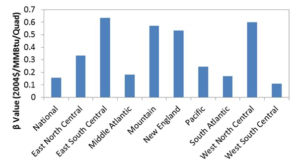
Fig. 63 \(\beta\) values for the nine census divisions.
The “National” value at the far left is \(\beta_{\text{nat}}\). A \(\beta\) of 0.2 means if demand increases by 1 quad, the price will increase by $0.20/MMBtu (see (1)).
The \(\alpha\) terms are then regressed for each scenario assuming the same \(\beta\) values for all scenarios. Although the \(\beta\) terms are derived from AEO2014 data, \(\alpha\) terms are regressed using the most recent AEO data. Thus, we assume natural gas price elasticity has remained constant, whereas price projections shift over time as represented by the \(\alpha\) values.
Comparison of Elasticities From Regression Approach to Literature Values
Technical literature tends to report the price elasticity of supply and the price elasticity of demand, which are estimates of the supply and demand, respectively, of a good given a change in price. In the formulation given by (1), we attempt to estimate a value that is similar to the price elasticity of demand—we estimate a change in price given a change in demand. Therefore, we present here a comparison against the price elasticity of demand as the closest available proxy, noting it is not necessarily identical to estimates of \(\beta\). Price elasticity of demand is typically negative but is reported here as a positive number for convenience.
External sources are varied and often vague in their estimates of price sensitivity of natural gas. Using the reported domestic NG market demand given for 2012 in AEO2014, the \(\beta\) values reported here yield an overall NG sector elasticity value of 0.36–0.92 (higher values of \(\beta\) correspond to lower elasticity values). Arora 2014 estimated the price elasticity of demand for NG to be 0.11–0.70, depending on the granularity and time horizon of the NG price data considered. Bernstein and Griffin 2006 examined the price elasticity of demand for residential NG usage, and they estimated the long-run elasticity to be 0.12–0.63 depending on the region. The Energy Modeling Forum at Stanford University reports NG price elasticity of demand for 13 energy models [Huntington, 2013]. The reported elasticity ranges from 0 to 2.20, depending on the year, model, and scenario considered. For the NEMS model, which is used for the AEO, the elasticity ranges from 0.22 to 0.81, depending on the year and scenario [Huntington, 2013].
EPA’s proposed Clean Power Plan included a projection that natural gas usage will increase by 1.2 quads in 2020, resulting in an 8%–12% increase in NG prices for the electric sector [Smith, 2014]. This corresponds to a \(\beta_{\text{nat}}\) of 0.38–0.51 in 2004$/MMBtu/quad.
Constant Elasticity of Supply
The second method for representing gas price adjustments leverages a constant elasticity of supply curve for census division prices as a function of the quantities consumed. The general form of the equation relies on a reference price (\(\overline{p}\)), a reference quantity (\(\overline{q}\)), and a price elasticity of supply (\(\epsilon\))[39] to determine the endogenous price (\(p\)) based on an endogenous quantity (\(q\)) so:
When parameterizing for the census division representations, the supply curve should reflect the change in price given a change in the census division’s quantity consumed in the electricity sector. To the best of our knowledge, no published studies estimate the elasticity of supply for natural gas specific to each sector and region. Therefore, the calibrated curve must consider the change in the census division’s price given a change in the consumption of natural gas in the region’s electricity sector with respect to other regions and sectors. To do this, the reference price, numerator, and denominator in the previous equation are adjusted to reflect the consumption change only in the electricity sector. Explicitly, the constant elasticity of supply parameters are now indexed by census division (\(r\)) and sector \(s \in \{ electricity,\ \ industrial,\ \ residential,\ \ commercial,\ \ vehicles\}\)). The equation used to populate the supply curve in the model becomes:
A potential addition to this representation, included as a switch in the model, also includes national price adjustments as deviations from the reference point. By denoting the national price as \(p_{ele,nat}\), the deviation from the benchmark price based on national quantities consumed in the electricity sector can be computed as:
Seasonal Natural Gas Price Adjustments
We use natural gas futures prices to estimate the ratio of winter to nonwinter natural gas prices to implement seasonal gas price differences in ReEDS. We chose futures prices for two reasons: ReEDS represents a system with no unforeseen disturbances, which is similar to futures prices, and historical natural gas prices have fluctuated greatly since the deregulation of natural gas prices.
Fig. 64 shows the cyclical nature of the natural gas futures prices. Fig. 65 separates the same prices into seasons, showing the nonwinter seasons have nearly the same price whereas wintertime prices are consistently higher. Wintertime prices are on average 1.054 times higher than nonwinter prices. The standard deviation of this price ratio is 0.004, indicating the ratio shows very little year-to-year variation.
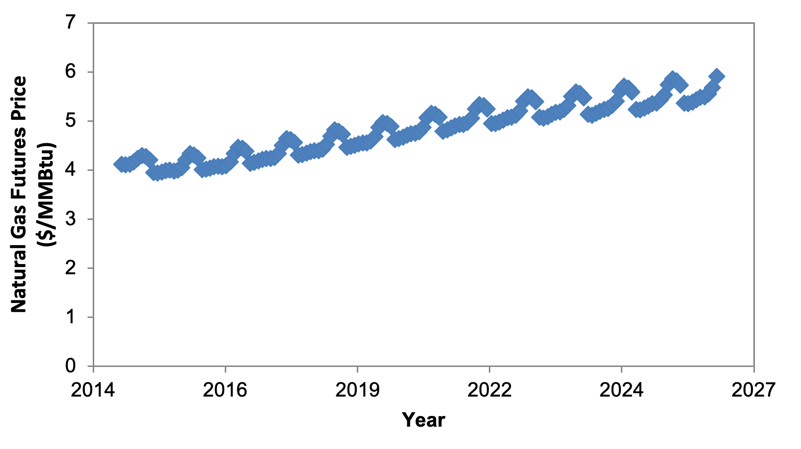
Fig. 64 Natural gas futures prices from the New York Mercantile Exchange for July 10, 2014.
The prices show the higher wintertime prices and the cyclical nature of the prices.
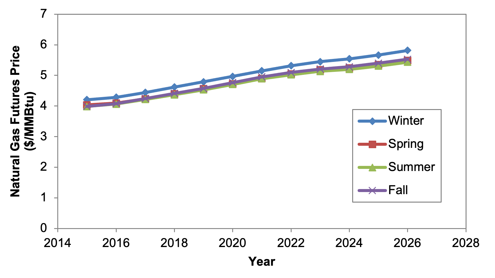
Fig. 65 Natural gas futures prices from Fig. 64 separated by season.
A seasonal natural gas price multiplier is calculated in ReEDS based on the natural gas price ratio so wintertime prices are 1.054 times higher than nonwinter prices without changing the year-round average price. Mathematically, this can be expressed as:
where \(P\) is the natural gas price for the period indicated by the subscript, \(W_\text{winter}\) is the fraction of natural gas consumption that occurs in the winter months, and \(\rho\) and \(\sigma\) are the seasonal multipliers for winter and nonwinter, respectively. The multipliers \(\rho\) and \(\sigma\) are determined by solving (2) through (5).
Capital Cost Financial Multipliers
The financial multiplier represents the present value of revenue requirements necessary to finance a new investment, including construction financing, return to equity holders, interest on debt, taxes, and depreciation. The formula is based on [Short et al., 1995] and is given by:
where \(\text{ConstCostMult}\) is the construction cost multiplier (the additional cost to finance construction), \(\text{FinancingMult}\) is the financing multiplier (adjusts required returns for diversifiable risk), \(\text{PresentValueDepr}\) is the depreciation expense (reduces the taxable income and is itself reduced by the investment tax credit), \(\text{ITC}_\text{eff}\) is the investment tax credit, and \(T\) is the tax rate.
Construction Cost Multiplier: The construction cost multiplier (\(\text{ConstCostMult}\)) captures the cost to finance the construction of the plant at construction interest rate \(i\). We use a midyear discounting and account for the deduction of interest payments for taxes.
The derivation of the construction cost multiplier is given below.
The total payment (\(\text{TotalPayment}\)) required to finance \(x\) fraction of construction investment (\(\text{Inv}\)) at interest rate \(i\) in construction year \(t\)—where \(t\) is defined relative to the in-service date (\(t=0\) is the final year of construction; \(t=1\) is the penultimate year of construction; etc.)—is the following:
Define the interest payment (\(I\)) in year \(t\) as a function of the total payment (\(\text{TotalPayment}\)) and the principal payment (\(P\)):
The tax savings (\(S\)) from interest deductions in year \(t\) at tax rate \(T\) is equal to:
Therefore, the absolute net change in the investment cost because of construction financing is the interest payments less the tax savings:
Finally, the total relative change in the investment cost because of construction financing is:
Financing Multiplier: The financing multiplier (not to be confused with the financial multiplier) is an adjustment to reflect either higher or lower returns to capital, relative to the systemwide average return to capital. Conceptually, it is a multiplier that reflects the total present value of a stream of higher (or lower) payments to capital, relative to what the payments would be at the system’s average cost of capital. For example, if a technology’s weighted average cost of capital (\(\text{WACC}_\text{tech}\)) is 7% and the systemwide WACC is 5% (\(\text{WACC}_\text{sys}\)), and the technology is being evaluated for a 20-year horizon (\(l\)) at a real discount rate of 5% (\(d_r\)), the financing multiplier (\(\text{FinancingMult}\)) would be 1.25, according to the equation below. This multiplier represents that the total present value of the returns to capital for this technology must be higher (by an amount equal to 25% of the initial investment), relative to a technology with average financing terms. The difference in the technology WACC and systemwide WACC represents the difference in returns to capital because of diversifiable risk.
To derive the above equation, begin with the definition of the capital recovery factor (\(\text{CRF}\)) for real discount rate (\(d_r\)) and economic horizon (\(l\)):
Therefore, for every dollar invested in a technology, the absolute difference in required return is:
Finally, the relative difference in required return per dollar invested is:
Depreciation Expense: The present value of depreciation (PVdepr) expense is computed based on the fraction of the plant value that is depreciable in each year. All investments use a MACRS depreciation schedule with \(f_t^\text{depr}\) representing deprecation fraction in year \(t\). This depreciation is sheltered from taxes, which is reflected by the term \(1 - T \cdot \text{PresentValueDepr}\) in the financial multiplier equation above.
Depreciable Basis: The eligible cost basis for MACRS depreciation expense is reduced by one-half the effective value of the tax credit:
Investment Tax Credit: The value of the ITC is reduced to reflect the costs of monetizing it (\(m_\text{ITC}\)). The effective investment tax credit value (\({ITC}_{eff}\)) reduces the tax burden of the investments.
Taxes: The denominator term of the financial multiplier equation (\(1-T\)) reflects the additional revenues necessary to pay taxes. The tax burden is adjusted for depreciation expenses as well as the effective investment tax credit.
Weighted Average Cost of Capital: The technology-agnostic nominal discount rate \(d_n\) is represented as the average WACC where \(d_f\) is the debt fraction, \(\text{RORE}_n\) is the nominal rate of return on equity, \(T\) is the effective tax rate, and \(I_n\) is the nominal interest rate on debt:
Calculating Present Value of Direct Electric Sector Cost
The equations in this section are used to calculate the present value cost of building and operating the system for some defined economic analysis period. To calculate the present value of total system cost, the cost in each future year \(t\) is discounted to the initial year of the economic analysis period, \(t_0\), by a social discount rate, \(d_\text{social}\). The real social discount rate used here for present value calculation is different from the investment discount rate assumptions, or cost of capital (WACC) assumptions.
The present value, or \(\text{PresentValue}\) in the equation, comprises two cost components: the present value of all operational costs in the model for the analysis period, \(\text{PresentValue}^\text{op}\) (including fixed and variable operating and maintenance costs for all sectors and fuel costs) and the present value of all new capital investments, \(\text{PresentValue}^\text{cap}\).
The present value of energy system costs is then calculated as:
Operational costs, \(\text{PresentValue}^\text{op}\), and capital costs, \(\text{PresentValue}^\text{cap}\), are discounted from year \(t\) by \(\frac{1}{\left(1 + d_\text{social} \right)^{t - t_0}}\) for each year in the analysis period:
where \(C_t^\text{op}\) is the operational costs in year \(t\) and \(C_t^\text{cap}\) is the capital costs in year \(t\). For all ReEDS system cost results, we assume the operational costs for the nonmodeled year are the same as the closest model year.
Marginal Electricity Prices
The marginal electricity prices in ReEDS are taken as the shadow prices from the constraints in the model that are directly impacted by the need to serve electricity. These include the load balance constraint, the operating reserve requirement, the RPS and CES requirements, and the planning reserve margin requirement (applied either in stress periods or seasonally via capacity credits). Taken together, these values show the total marginal cost of serving electricity in a given region and time slice. Weighted average versions are also calculated to report national annual marginal electricity prices. These marginal prices are most analogous to wholesale electricity prices but within a model that has full coordination and foresight.
Marginal Price Outputs
Marginal electricity price outputs are calculated with reqt_price in e_report.gms and are outputs in reqt_price.csv. The quantity required by the model is reported in the reqt_quant.csv output. These two taken together can be used to calculate a $/MWh electricity price, which is done in make of the ReEDS outputs and reported as “Bulk System Electricity Price” in bokehpivot HTML outputs and in other output locations.
Average Electricity Prices
Average electricity prices are calculated as the annualized total costs of building and operating the system in a certain geographic area, divided by the electricity load in that area. At the national level, the prices are calculated as:
where system costs include both annualized capital and operational costs. Annualized costs for existing (i.e., pre-2010) power plants are also considered given plants’ initial investment costs and the build year.
At the zonal level, average electricity prices also consider the impact of energy and capacity trading:
Where n, p, and zone all indicate model zones; \(import_{n,p,h,t}\) indicates energy or capacity transfer from n to p; and \(export_{p,n,h,t}\) indicates energy or capacity transfer from p to n. Capital costs also include annualized costs for pre-2010 power plants.
Specifically, the energy import/export is calculated as:
where t is year, p and n are both model zones, and h indicates time slices.
Interday Storage Operation
Interday linkage must be established for LDES.
Simulating LDES requires interperiod linkage to reflect seasonal SOC changes.
This can be achieved by using a fully chronological year at hourly resolution with GSw_HourlyType = 'year', but this approach is computationally intensive.
Alternatively, ReEDS offers an interday linkage option that enables SOC linkage across representative days while maintaining high computational efficiency.
This interday linkage can be activated using GSw_InterDayLinkage, which is designed to work with the representative day and week method (GSw_HourlyType = 'day' or 'wek').
Without the interday linkage, SOC is typically limited to intraday changes and resets at the end of each representative period, preventing interperiod variations.
However, with interday linkage enabled, SOC can evolve across multiple periods, with fidelity improving as the number of representative periods increases, as demonstrated in Fig. 66.
The interday linkage is built using a sparse chronology strategy—a recently developed method that is computationally efficient and accurate—as referenced in [Chen et al., 2024].

Fig. 66 Comparison of the state of charge of a 100-hour battery across different temporal cases and numbers of representative days.
Storage Capacity Credit
Resource adequacy modeling in ReEDS uses the stress periods approach by default, which uses the same model for storage as described in the temporal resolution section. Here the treatment of storage under the alternative capacity credit method is described.
The storage capacity-credit method characterizes how much energy duration is required to serve peak demand as a function of total storage power capacity. The potential of storage to serve peak demand is considered by performing several simulated dispatches against the load profiles within each of the resource assessment regions. Net load profiles of wind and PV generation are used to capture the effects of VRE resources on the overall net load profile shape in a region using the hourly load, wind, and solar profiles.
For each season and reliability assessment zone, storage dispatch is simulated with peaking capacity prioritized over all other services (reflecting capacity market prioritization as discussed by [Sioshansi et al., 2014]). Transmission constraints are ignored within each reliability assessment zone; this copper plate transmission assumption applies only to the capacity credit calculation—all transmission constraints are enforced in the actual planning reserve margin constraint and other system planning and operation modeling in ReEDS. Optimal coordination of dispatch among energy storage resources is also assumed. The transmission and coordination assumptions together allow for all storage within a reliability assessment zone to be represented as a single aggregate resource. The round-trip efficiency of this aggregated storage resource is assumed to be equal to the energy-capacity-weighted average round-trip efficiency of all installed storage capacity in that region.
Round-trip efficiency losses are included in storage charging. For example, a storage resource with a round-trip efficiency of 85% and a power capacity of 10,000 MW can dispatch 10,000 MW to the grid for 1 hour using 10,000 MWh of energy capacity. However, when the same resource draws 10,000 MW from the grid for 1 hour, its SOC increases by only 8,500 MWh.
Fig. 67 illustrates the dispatch and calculation of the energy requirement for 5,000 MW of storage to receive full capacity credit in the New York Independent System Operator (NYISO) region in 2020. First, the storage power capacity is subtracted from the peak load to set a net load maximum. Storage is required to discharge whenever the load profile exceeds this maximum to ensure the peak net load (load minus storage, in this example) is equal to the peak load minus the power capacity of the storage device. The storage is allowed to charge at all other times while ensuring the load maximum is not exceeded.
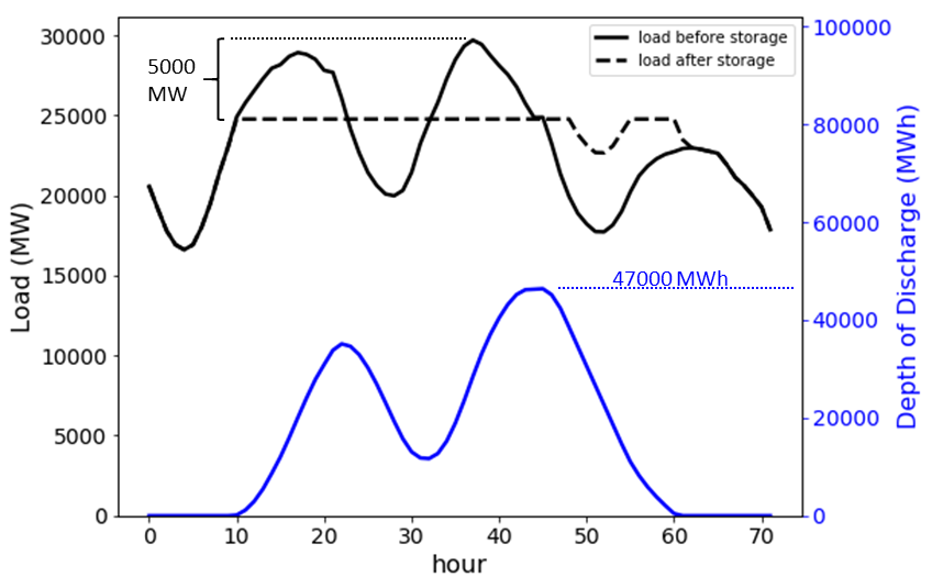
Fig. 67 Model results for determining energy capacity requirements for storage in NYISO in 2020 for a 3-day example in August. 47,000 MWh is determined to be the necessary energy capacity for 5,000 MW of storage to receive full capacity credit. A depth of discharge of 0 indicates the storage is full.
This dispatch is then used to calculate the energy requirement for storage to receive full capacity credit. At the beginning of the season, the SOC of storage within the region is assumed to be full. The state of charge (or depth of discharge, as is shown in Fig. 67) is tracked over the course of the time series with the maximum depth of discharge left unconstrained. This means the maximum depth of discharge value over the course of the season is equal to the amount of energy capacity that is needed for storage to receive full capacity credit. Dividing this energy by the power capacity used produces the minimum fleetwide average duration (hours) for storage to receive full capacity credit. In the example in Fig. 67, 5,000 MW of peak demand reduction from storage would require 47,000 MWh of energy to receive full capacity credit, or a duration of 9.4 hours.
We repeat this process in each region for each season over a large range of storage power capacities (from 0% to 90% of peak demand in 100-MW increments). The result of each dispatch is used to produce the “power-energy curve” in Fig. 68, which allows us to calculate the marginal capacity credit for additional storage. The curve gives storage energy capacity that is required for full capacity credit as a function of total storage capacity.[^ref45] At any point along the curve, the slope of the tangent to the curve represents the number of hours needed for marginal storage to receive full capacity credit. The incremental capacity credit of an additional unit of storage is equal to the duration of the additional unit installed divided by the duration requirement (slope) at the point on the curve corresponding to the installed storage capacity.
The storage capacity credit method in ReEDS characterizes how much additional storage duration is needed to serve peak demand as storage penetration increases. The power-energy curve acts as a constraint, in which the power value is treated as the firm capacity contributing to resource adequacy. To ensure there is always enough energy to support the targeted demand reduction, the combined storage power and energy capacities must lie above the power-energy curve.
One challenge for ReEDS is that it is a linear model, whereas the power-energy curve is nonlinear. To address this, a binning method is used to develop a piecewise, linearized power-energy curve. This process differs between discrete-duration and continuous-duration storage technologies. For discrete-duration technologies, storage duration bins are predefined, and the power-energy curve is linearized using the slopes associated with these storage durations. The power bin sizes for each bin, determined by the intersection of the power-energy curve with the corresponding predefined duration slopes, are output to represent the minimum storage duration required to achieve the desired demand reductions while ensuring sufficient energy supply.
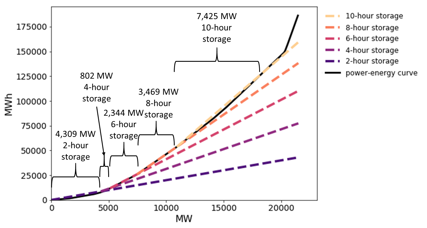
Fig. 68 Example power-energy curve and the binning logic. The power-energy curve represents the energy capacity need for expected demand reduction given the load profile. The five storage bins (sdbin) are the default ReEDS setup, and the storage bin size (sdbin_size and sdbin_size_energy) are the crossover of the storage bin slopes with the power-energy curve, representing the theoretical highest demand reduction capability of the bins and the corresponding energy capacity needed, used as the constraints for ReEDS system sizing.
Discrete-Duration Framework
Discrete-duration battery framework was previously applied to discrete-duration batteries and is currently used for pumped hydro. In this approach, stand-alone storage must be allocated to predefined storage bins. This allocation is calculated in following equations, using the sets I, R, T, and SDBIN, where I represents generation technologies (focused here on stand-alone storage), R refers to ReEDS regions, T denotes model years, and SDBIN defines the preassigned storage duration bins.
By default, ReEDS uses bins of 2, 4, 6, 8, 10, 12, 24, 48, 72, and 100 hours, along with an overflow bin at 8760 hours. CAP denotes the total generation capacity, whereas CAP_SDBIN refers to the capacity allocated by storage bin. Parameters are denoted in lowercase: sdbin_size represents the power capacity for each bin, based on the storage duration and the power-energy curve, indicating the maximum power the bin’s duration can support. cc_storage stands for the capacity credit applied to each storage duration, reflecting the discount in credited power when storage is placed in a higher-duration bin. For example, a 4-hour storage would receive full credit (1) in the 2- and 4-hour bins, but only 0.667 in the 6-hour bin and 0.5 in the 8-hour bin. To encourage allocation to shorter-duration bins first for instances when the constraint is not binding, ReEDS applies a very small penalty to the objective cost when storage is placed in longer-duration bins. Additionally, peakdemand represents the peak demand requirement, prm is the planning reserve margin, and X represents other firm capacities that contribute to resource adequacy.
The first equation ensures the binned power capacity, adjusted by capacity credit, does not exceed the corresponding storage bin size; otherwise, there would not be enough energy to support the intended demand reduction. The second equation requires that the binned power capacity used for capacity credit must be greater than or equal to the actual power capacity. This ensures the existing storage resources are properly allocated and sufficient to meet the capacity needs of each storage bin. Together, the first and second equations linearize the power-energy curve and allocate storage capacity to meet its requirements, effectively translating actual power capacity into storage bin capacity for firm capacity contributions. The third equation represents the final constraint for meeting demand reduction: the total storage bin capacity from stand-alone storage technologies, combined with other firm capacity, must be greater than or equal to peak demand plus the planning reserve margin.
Continuous-Duration Framework
The continuous-duration framework is currently applied to lithium batteries. Since the storage duration in this framework is not fixed, we introduce two additional equations to support the continuous framework, in addition to the three equations above.
Using this approach, the first equation links the power and energy constraints for each storage bin, calculating the energy required to meet the demand reduction associated with that bin (as sdbin_size_energy shown in Fig. 68). The second equation then enforces a minimum battery energy capacity, ensuring the storage technology is sufficiently sized to support the peak reduction. As a result of these two equations, the capacity credit (cc_storage) in this case is effectively always equal to 1. This schematic enables the integration of continuous-duration framework into the storage bin and capacity credit framework, allowing them to function effectively within the model.
Storage capacity credit is sensitive to a variety of factors on the power system, so, rather than ignoring the many factors that can influence storage capacity credit, we simply pass the model information on what storage could do to serve peaking capacity based on load shape and storage duration and then allow the model to choose the least-cost option based on the suite of available resources and the entire set of storage revenue streams represented within the ReEDS model. Interactions between the storage peaking potential of storage and VRE generation fraction are described by [Denholm et al., 2019, Frazier et al., 2020].
The capacity credit of CSP with storage is calculated using the same method as other storage technologies, except rather than using net load to show opportunities to charge, DNI resource is used to show opportunities to charge the storage.
Spatial Resolution Capabilities
The default model zones are shown in Fig. 18. Depending on the needs of the user, different spatial resolutions can also be used. The default zones can be aggregated into larger regions, or collections of zones can be disaggregated into their constituent counties (Fig. 69). National-scale county-level resolution runs are extremely computationally intensive and require simplifications in other aspects of the model (e.g., fewer time steps, solve years, or technologies) to be able to produce a solution—even with simplifications, hundreds of gigabytes of memory are required to process the county-level inputs. Runs that aggregate zones across state boundaries require state policies be turned off because the model does not have any built-in features for aggregating state policies for states that have been combined.
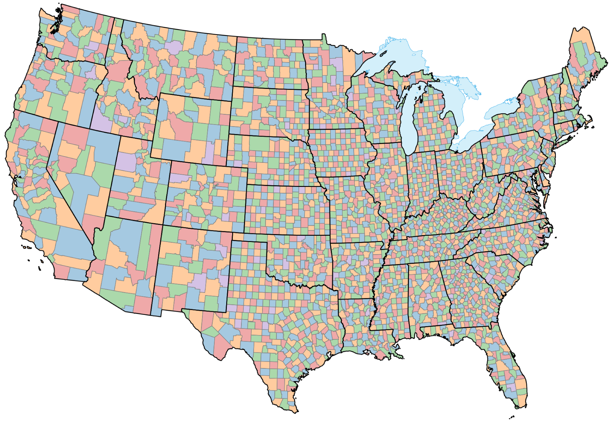
Fig. 69 Counties of the contiguous United States.
The spatial framework built into the ReEDS model allows other spatial resolutions or spatial extents; for example, ReEDS has been used to represent the RTS-GMLC nodal test system [Karmakar and Cole, 2024] and the zonal Indian power system [Joshi et al., 2024, Rose et al., 2020]. When running with nodal data, each renewable energy resource site can be associated only with a single node, so the node assignments must be done before a model run is performed. And regardless of spatial extent or resolution, all decision variables will still be linear.
The model also has the capability to use mixed resolutions. For example, California can be represented using the default model zones, whereas the rest of the United States is represented at state resolution. This can enable finer detail for a specific region of interest while capturing trades with neighboring regions at lower resolution but with a reasonable solution time.
Data inputs and handling
Nearly all ReEDS data inputs that include a spatial dimension are specified at the 134-zone model resolution.[40] To be able to perform runs at county-level resolution, some inputs are included at both the county level and zonal resolution.
Transmission data
Transmission capacity between counties is based on nodal transmission network data (see Fig. 70) collected as part of the North American Renewable Integration Study [Brinkman et al., 2021]. Nodes from the dataset are spatially matched to counties using nodal coordinates and a shapefile of U.S. counties (described below). With this dataset, there are a few dozen counties that have no transmission nodes or capacity, which may be the result of missing data (the quality of the nodal dataset declines for lower-voltage (less than 100 kV) transmission elements). To address this, nodes and lines are added to ensure every county has at least one transmission interface. This is done by either adding a node on existing lines that cross a county but previously had no nodes in that county, or, if there are no transiting lines, adding a node to the county centroid and connecting to the closest node in a neighboring county.
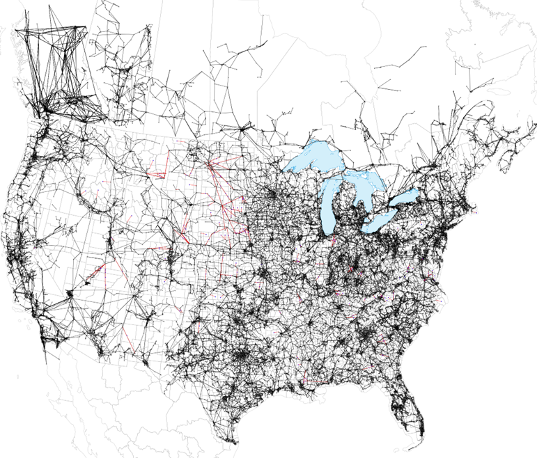
Fig. 70 Nodal transmission network data. Black lines are those from the dataset, and red lines are the lines that were added to ensure every county included at least one interface.
Power flow constraints imposed by the topology of the network can limit the true transfer capacity between two counties to a level below the physical capacity of the lines connecting those counties. ReEDS estimates these interface capacity limits using an optimization method that finds the maximum transfer values given network characteristics, the location of generators and load, and other constraints [Brown et al., 2023]. Because interface limits are typically less influenced by parts of the network that are farther away, the method is run on a subset of the network. This subset is selected by including all parts of the network that are a specified number of “hops” away from the interface being optimized. A comparison of the results from the optimization method with different hops found total transfer capacity saturated after six hops, so this value was used when calculating the county-level transfer limits used in ReEDS. Because the transfer capacity can differ depending on the direction, the optimization is run once in each direction (forward and reverse) for each interface. Further information on the development of county-level transmission interfaces is provided by [Sergi et al., 2024]
After the optimization, some counties have zero transfer capacity in one or both directions; these are replaced with either the transfer capacity estimated in the other direction if it is nonzero or with the thermal capacity of the line. To estimate metrics such as TW-mi of transfer capacity, ReEDS uses the distance between the centroids of the two counties in the interface. Following this adjustment, we find some counties still have a supply (and transmission import capacity) shortfall compared to their demand in historical years. The source of the shortfall is likely due to a combination of demand disaggregation from BA to county scale and underestimation of county transmission due to the importance of lower voltage transmission and sub-transmission for county level connectivity. This shortfall will artificially reduce the resource adequacy for existing years and will also force immediate investments which only serve to bridge this gap. Therefore we perform a least-cost transmission capacity expansion model across stress timeslices which allows investment in new capacity on existing transmission lines or build new lines at a premium if absolutely required. This opertion is being performed by the code located in the ReEDS-2.0_Input_Processing Repository Users should use this transmission dataset as a baseline from which to begin county level analysis rather than a perfect fidelity county-county transmission map. Additional county level caveats are provided in the section on spatial resolution. The final transmission limits calculated using this method are shown in Fig. 71.
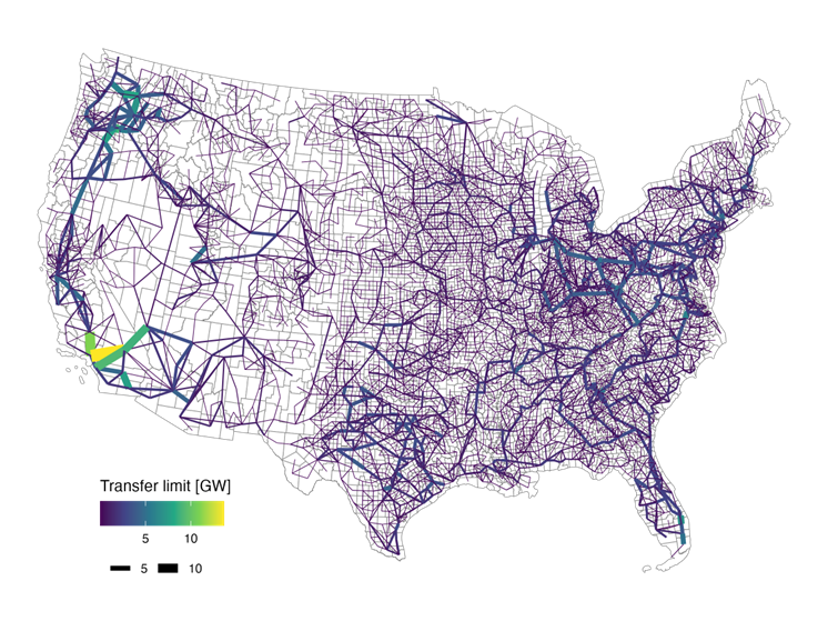
Fig. 71 Final transfer limits used in the county-level input dataset for the forward direction.
Except for a small number of predetermined lines, all AC expansion options at county resolution are limited to 250 miles in order to limit the number of possible expansion pairs.
Wind and solar supply curve data
Supply curves for wind and solar are based on data from the reV model, which provides total resource potential, representative resource profiles, and any location-dependent supply curve costs [Maclaurin et al., 2021]. Each supply curve point from the reV model is mapped directly to its corresponding county. These supply curve points are then aggregated by ReEDS to produce county-level supply curves.
The reV model includes estimates of the cost of investments needed to reinforce the transmission network with the addition of more wind and solar. For the ReEDS zonal spatial representation, these network reinforcement costs are calculated by determining the least-cost interconnection point and then estimating the transmission upgrades needed between that point and the zone’s network node. Because the county-level resolution now explicitly represents transmission investments between counties, the network reinforcement costs from reV are not included in the transmission cost estimates of the county supply curves. Spur line costs, or the cost to build from the resource site to the interconnection point, are still taken from reV. In the future, the reV model may be adapted to produce network reinforcement costs at the county level, although they might be sufficiently small that ignoring them would be appropriate. POI costs are still represented at county resolution.
Power plant capacity data
Capacity data in ReEDS for existing units, prescribed builds, and prescribed retirements[41] are taken from the NEMS power plant database. The power plants in this database include latitude and longitude to give their location. These locations are mapped to counties to provide the county assignment for the power plants. In a few isolated cases, hydropower units that were on a county boundary were manually assigned to a county to better align with the transmission infrastructure that connects the plant to the rest of the electricity system.
Shapefiles
Matching transmission nodes to counties and plotting maps of county-level results requires shapefiles of U.S. counties. For this purpose, ReEDS relies on the 2022 vintage of TIGER/Line Files published by the U.S. Census Bureau, which includes all legal boundaries and names as of January 1, 2022 [U.S. Census Bureau, 2022]. The shapefiles are converted to the ESRI:102008 coordinate reference system, and any counties outside the CONUS are dropped.
Scaling datasets to county resolution
All datasets besides those described above were downscaled from 134-zone resolution to county-level resolution using one of the following three methods.
Uniform disaggregation:
All counties within a model zone are assigned the same value as the one used for the zone.
Downscaling based on population:
The “population” disaggregation method uses population fractions as multipliers to calculate county-level data from zonal inputs. The multipliers used in this method represent the fraction of a county’s population with respect to its corresponding ReEDS zone. Population data used to create the multipliers are sourced from the 2021 Population Totals dataset provided by the U.S. Census Bureau. Example data for ReEDS Zones p29 and p30 are shown in Table 29.
ReEDS Zone |
County |
Population Fraction |
|---|---|---|
p29 |
p04001 |
1 |
p30 |
p04019 |
0.956 |
p30 |
p04023 |
0.044 |
Because only one county exists in ReEDS Zone “p29,” the population fraction for that county is 1. On the other hand, two counties exist in ReEDS Zone “p30”: The population fractions show 95.6% of the population of p30 lives in County p04019, whereas 4.4% of the population lives in p04023. To disaggregate by population, the dataset is mapped to zonal ReEDS input data and the population fraction is multiplied by the values of the zonal-level dataset.
Downscaling based on existing hydropower capacity:
The existing hydropower disaggregation method uses the fraction of existing hydropower capacity in a given county with respect to the total hydropower capacity of the county’s corresponding ReEDS zone as fractional multipliers for downscaling zonal input data to county level. Existing hydropower capacity data used to calculate these fractional multipliers are sourced from the EIA-NEMS generator database included in the ReEDS inputs. This downscaling method is used for hydropower-specific data, such as hydropower upgrades.
We selected one of the three downscaling methods above for each of the inputs that included a spatial dimension and did not have a separate county-specific input file. The choice was made using analyst judgment. In the input structure of ReEDS, if an appropriate county-level dataset becomes available, it can be used in place of the downscaled dataset.
Input data handling
Because some input data are specified at both zonal and county resolution, the inputs used for a given run will depend on the spatial resolution selected for that run. The input scripts include logic that will read in the file with the appropriate spatial resolution and use that for the remainder of the run. In the case of mixed resolutions, both files will be read in, and the appropriate regions will be concatenated to create a single input file with the specified spatial resolutions.
ReEDS has been set up to run so only data for the regions being modeled will be included in the model. For example, if doing a run that includes only the state of North Dakota, the inputs processing step of ReEDS will filter all input data to include only the data for North Dakota.
Spatial datasets are dynamic within the model itself, so the model is agnostic to the region names.
Challenges and benefits of enhanced spatial resolution
The greater spatial resolution available in ReEDS with county-level inputs creates a variety of opportunities to apply the ReEDS model to answer questions. It enables specific regions of the country to be captured to greater resolution, enabling more granular outputs of power plant siting, transmission expansion, and emission impacts. The higher resolution can also highlight key regional boundaries or interfaces that might not have been present in a lower-resolution model run. County-level resolution can lead to better estimates of curtailment because there is more detail on the underlying transmission system [Serpe et al., 2025].
The enhanced spatial resolution also comes with a variety of challenges and limitations. These include:
Input data: Higher resolution datasets can have gaps or limitations that might not be apparent at coarser spatial resolution. For example, the transmission dataset discussed above does not have complete coverage at sub-transmission voltages (below 100 kV) and does not include distribution-level data, leading to unrealistic islanding of several counties.
Down-scaling approaches: Downscaling coarse-resolution datasets to the county level can lead to county-level datasets that are more smooth or less accurate than they would be in reality. For example, load data that is down-scaled to counties is likely to be more smooth than actual load profiles for that county, and the population-based weighting applied will not fully capture the distribution of loads within a larger region.
Linear modeling: At higher spatial resolution, the linear programming approach used by ReEDS can be insufficient. For example, ReEDS might choose to build a 3 MW gas plant in a county, but the ReEDS input costs are based on much larger power plants, so ReEDS would be underestimating the cost of that small plant (note that this is still an issue when using larger regions, but with larger regions small buildouts are much less common).
Transmission investments: ReEDS transmission investment costs are based on 500 kV transmission lines, but most counties in the U.S. are only connected at much lower voltage levels; many counties are only connected by transmission lines of less than 100 kV. Transmission costs increase on a per-MW basis as voltage declines, so county-level transmission costs will in general be higher than estimates based on 500 kV lines. Expansion of transmission lines in ReEDS represents electricity transfer bottlenecks that ReEDS sees valuable to expand rather than investments in specific transmission lines or corridors.
Transmission flows: ReEDS uses a pipe-and-bubble approach for transmission flows, which loses accuracy at higher spatial resolution. Existing interface transfer limits at the county level are calculated using a nodal DC powerflow model as described above, and the resulting ITLs are treated as superimposable within ReEDS (i.e., the flow on one interface does not affect the flow on other interfaces). [Brown et al., 2023] shows that ITLs for larger interfaces (for example, between ISOs) tend to be smaller than the sum of ITLs of constituent interfaces. The sum of individual county ITLs may thus overstate coincident flow limits. [Mehrtash et al., 2023] shows the choice of transmission power flow representation can have a significant impact on the model solution.
False precision: When running ReEDS at high spatial resolution, outputs will naturally be reported at that level of resolution. Users are cautioned against putting more stock into a particular model solution than is warranted because of uncertainty in the data or methods used. For example, moving new capacity from one county to a neighboring county might have almost no impact on total system cost and therefore be an equivalent solution to the one reported by ReEDS.
Runtime: Much of our testing showed a tenfold increase in the number of regions led to at least a tenfold increase in solve time, although runtime ultimately depends on the machine specifications and the model options selected for that particular run [Serpe et al., 2025]. Although national-scale runs are possible with enough simplifications, county-level resolution is typically only used to model much smaller regions.
Running ReEDS Beyond 2050
By default most of the ReEDS input datasets are exogenously provided up to the year 2050, thus defining the default maximum end year for model runs. ReEDS can also extending its year-indexed datasets beyond 2050 using a variety of “forecasting” extrapolation methods determined by user-defined assumptions about the future behavior of the data. This dataset “forecasting” allows ReEDS to then be be solved to any future model year beyond 2050 at up to 10-year timesteps.
Forecasting Methods
Two methods can be used to extrapolate year-indexed datasets: the last year’s data can be extended at a constant level, or the final years of data can be fit with linear regression and extended at a constant slope.
Constant
This method copies the last available year of data for all future model years up to the post-2050 model endyear.
Linear Regression
This method linearly forecasts post-2050 data based on the last “x” years of available data, where “x” is a user-defined number of years to include in determining the slope for linear extrapolation. For now only 5-year and 10-year linear regressions are used, though any number of years can be used in regression calculations.
This method requires annual data in determining the extrapolation slope - thus, data is first interpolated to fill any missing year. For example, if extrapolating data beyond 2050 using a 5-year linear method then this method will interpolate any missing 2046, 2047, 2048, 2049, and 2050 data before calculating the extrapolating slope. Once calculated, this slope is then used to calculate data for all model years beyond 2050.
ReEDS Model Contributors
All NREL contributors to the ReEDS model are listed below.
Abdelrahmam Ayad
Jon Becker
Ross Beppler
David Bielen
Nate Blair
Max Brown
Patrick Brown
Vincent Carag
Yunzhi Chen
Stuart Cohen
Wesley Cole
Sean Corcoran
Paul Denholm
Victor Diakov
Victor Duraes de Faria
Kelly Eurek
Will Frazier
Bethany Frew
Rebecca Fuchs
Nathaniel Gates
Danny Greer
Sameera Gudladona
Claire Halloran
Maureen Hand
Anne Hamilton
Donna Heimiller
Jonathan Ho
Eduardo Ibanez
Paige Jadun
Charles Kang
Akash Karmakar
Saroj Khanal
Venkat Krishnan
Katie Lamb
Anthony Lopez
Helen Lu
Scott Machen
Madeline Macmillan
Trieu Mai
Andrew Martinez
Dana Max
Maureen McDaniel
Kennedy Mindermann
Joseph Mowers
Matthew Mowers
David Mulcahy
Caitlin Murphy
John Nangle
Claire Nguyen
Scott Nicolson
Kodi Obika
Hyungseon Oh
An Pham
Andrew Reimers
James Richards
Anna Schleifer
Brian Sergi
Louisa Serpe
Shashwat Sharma
Sophia Shi
Walter Short
Ben Sigrin
Travis Simpkins
Ramteen Sioshansi
Elina Spyrou
Ragini Sreenath
Dan Steinberg
Patrick Sullivan
Aaron Townsend
Merve Turan
Caroline Uriarte
Max Vanatta
Nina Vincent
Tibebe Woldeyesus
Ella Zhou
Owen Zinaman
Matt Zwerling