Fuel Property Prediction Model

FuelLib utilizes the group contribution method (GCM), as developed by Constantinou and Gani[1] [2] in the mid-1990s, to provide a systematic approach for estimating the thermodynamic properties of pure organic compounds. The GCM decomposes molecules into structural groups, each contributing to a target property based on predefined group values. By summing these contributions, the GCM accurately predicts essential properties, including the acentric factor, normal boiling point, liquid molar volume at standard conditions (298 K) and more. This predictive capability is particularly useful for complex mixtures such as synthetic aviation turbine fuels (SATFs), where experimental thermodynamic data is limited. FuelLib provides SATF developers with a means to estimate these critical properties without extensive physical testing, thereby aiding in the identification of promising fuel compositions before committing to large-scale production.

FuelLib builds on Pavan B. Govindaraju’s Matlab implementation, and includes gas chromatography data (GC x GC) for various jet fuels from the National Jet Fuel Combustion Program[3] (NJFCP) Air Force Research Laboratory[4] [5] (AFRL) and Vozka et al.[6]. Additionally, FuelLib includes correlations for the thermodynamic properties of mixture such as density, viscosity, vapor pressure, surface tension, and thermal conductivity. Table of GCM properties outlines the properties for the i-th compound in a mixture, which depends on the k-th first-order and j-th second-order group contributions.

Table of GCM properties

Table 1 GCM properties of the i-th component in a mixture. The subscript stp denotes a standard pressure assumption.

Property	Units	Group Contributions	Units	Description
\(M_{w,i}\)	kg/mol	\(m_{w1k}\)	g/mol	Molecular weight.
\(T_{c,i}\)	K	\(t_{c1k}\), \(t_{c2j}\)	1	Critical temperature[1].
\(p_{c,i}\)	Pa	\(p_{c1k}\), \(p_{c2j}\)	bar-0.5	Critical pressure[1].
\(V_{c,i}\)	m3/mol	\(v_{c1k}\), \(v_{c2j}\)	m3/kmol	Critical volume[1].
\(T_{b,i}\)	K	\(t_{b1k}\), \(t_{b2j}\)	1	Normal boiling point[1].
\(T_{m,i}\)	K	\(t_{m1k}\), \(t_{m2j}\)	1	Normal melting point[1].
\(\Delta H_{f,i}\)	J/mol	\(h_{f1k}\), \(h_{f2j}\)	kJ/mol	Enthalpy of formation at 298 K[1].
\(\Delta G_{f,i}\)	J/mol	\(g_{f1k}\), \(g_{f2j}\)	kJ/mol	Standard Gibbs free energy at 298 K[1].
\(\Delta H_{v,\textit{stp},i}\)	J/mol	\(h_{v1k}\), \(h_{v2j}\)	kJ/mol	Enthalpy of vaporization at 298 K[1].
\(\omega_i\)	1	\(\omega_{1k}\), \(\omega_{2j}\)	1	Acentric factor[2].
\(V_{m,\textit{stp},i}\)	m3/mol	\(v_{m1k}\), \(v_{m2j}\)	m3/kmol	Liquid molar volume at 298 K[2].
\(C_{p,i}\)	J/mol/K	\(C_{pA1_k}\), \(C_{pA2_k}\),…	J/mol/K	Specific heat capacity[7] [8].

Equations for GCM properties

The properties of each compound in a mixture can be calculated as the sum of contributions from the first- and second-order groups that make up the compound. For a given mixture, let \(\mathbf{N}\) be an \(N_c \times N_{g_1}\) matrix that represents the number of first-order groups in each compound, where \(N_c\) is the number of compounds in the mixture and \(N_{g_1}\) is the total number of first-order groups as defined by Constantinou and Gani[1][2]. Similarly, let \(\mathbf{M}\) be an \(N_c \times N_{g_2}\) matrix that specifies the number of second-order groups in each compound, where \(N_{g_2}\) is the total number of second-order groups. The total number of groups \(N_g = N_{g_1} + N_{g_2} = 121\). The GCM properties for the i-th compound in the mixture are calculated as follows[1] [2] [8]:

\[\begin{split}\begin{align*} M_{w,i} &= \bigg[\sum_{k = 1}^{N_{g_1}}\mathbf{N}_{ik}m_{w1k} \bigg] \times 10^{-3}, \\ T_{c,i} &= 181.28 \ln \bigg[ \sum_{k=1}^{N_{g_1}} \mathbf{N}_{ik} t_{c1k} + \sum_{j=1}^{N_{g_2}} \mathbf{M}_{ij} t_{c2j} \bigg],\\ p_{c,i} &= \Bigg( \bigg[ \sum_{k=1}^{N_{g_1}} \mathbf{N}_{ik} p_{c1k} + \sum_{j=1}^{N_{g_2}} \mathbf{M}_{ij} p_{c2j} + 0.10022\bigg]^{-2} + 1.3705\Bigg)\times 10^{5}, \label{eq:gcm-pc}\\ V_{c,i} &= \Bigg( \bigg[ \sum_{k=1}^{N_{g_1}} \mathbf{N}_{ik} v_{c1k} + \sum_{j=1}^{N_{g_2}} \mathbf{M}_{ij} v_{c2j} \bigg] -0.00435 \Bigg)\times 10^{-3}, \\ T_{b,i} &= 204.359 \ln \bigg[ \sum_{k = 1}^{N_{g_1}} \mathbf{N}_{ik} t_{b1k} + \sum_{j=1}^{N_{g_2}} \mathbf{M}_{ij} t_{b2j}\bigg],\\ T_{m,i} &= 102.425 \ln \bigg[ \sum_{k = 1}^{N_{g_1}} \mathbf{N}_{ik} t_{m1k} + \sum_{j=1}^{N_{g_2}} \mathbf{M}_{ij} t_{m2j}\bigg],\\ \Delta H_{f,i} &= \Bigg( \bigg[ \sum_{k = 1}^{N_{g_1}} \mathbf{N}_{ik} h_{f1k} + \sum_{j=1}^{N_{g_2}} \mathbf{M}_{ij} h_{f2j} \bigg] + 10.835\Bigg) \times 10^3,\\ \Delta G_{f,i} &= \Bigg( \bigg[ \sum_{k = 1}^{N_{g_1}} \mathbf{N}_{ik} g_{f1k} + \sum_{j=1}^{N_{g_2}} \mathbf{M}_{ij} g_{f2j} \bigg] -14.828 \Bigg) \times 10^3,\\ \Delta H_{v,\textit{stp},i} &= \Bigg( \bigg[ \sum_{k = 1}^{N_{g_1}} \mathbf{N}_{ik} h_{v1k} + \sum_{j=1}^{N_{g_2}} \mathbf{M}_{ij} h_{v2j} \bigg] + 6.829\Bigg) \times 10^3, \\ \omega_i &= 0.4085 \ln \bigg( \Big[ \sum_{k=1}^{N_{g_1}} \mathbf{N}_{ik} \omega_{1k} + \sum_{j=1}^{N_{g_2}} \mathbf{M}_{ij} \omega_{2j} + 1.1507\Big]^{1/0.5050} \bigg), \label{eq:gcm-omega}\\ V_{m,\textit{stp},i} &= \Bigg( \bigg[ \sum_{k=1}^{N_{g_1}} \mathbf{N}_{ik} v_{m1k} + \sum_{j=1}^{N_{g_2}} \mathbf{M}_{ij} v_{m2j} \bigg] + 0.01211 \Bigg)\times 10^{-3}, \\ C_{p,i} & =\bigg[\sum_{k=1}^{N_{g_1}} \mathbf{N}_{ik} C_{pA1_k} + \sum_{j=1}^{N_{g_2}} \mathbf{M}_{ij} C_{pA2_j} -19.7779\bigg] \nonumber \\ & +\bigg[\sum_{k=1}^{N_{g_1}} \mathbf{N}_{ik} C_{pB1_k} + \sum_{j=1}^{N_{g_2}} \mathbf{M}_{ij} C_{pB2_j} + 22.5981\bigg] \theta \nonumber\\ & +\bigg[\sum_{k=1}^{N_{g_1}} \mathbf{N}_{ik} C_{pC1_k} + \sum_{j=1}^{N_{g_2}} \mathbf{M}_{ij} C_{pC2_j} - 10.7983\bigg] \theta^2 \\ \theta &= \frac{T - 298.15}{700} \end{align*}\end{split}\]

Equations for individual compound correlations

This section presents correlations for physical properties that leverage the individual compound properties defined in Equations for GCM properties. These correlations make it possible to evaluate physical properties at non-standard temperatures and pressures, given that group contribution properties are only defined at standard conditions. Unless noted otherwise in the individual correlation, all units are assumed to be SI: length (m), mass (kg), time (s), temperature (K), mole (mol). The Reduced temperature quantities are used throughout this section for each compound i, provided \(T\) in K unless noted otherwise.

Table 2 Derived quantities and temperature corrections

Property	Units	Description
\(\nu_i\)	m2/s	Kinematic viscosity[9].
\(L_{v,\textit{stp},i}\)	J/kg	Latent heat of vaporization at 298 K[10].
\(L_{v,i}\)	J/kg	Temperature-adjusted latent heat of vaporization at 298 K[10].
\(V_{m,i}\)	m3/mol	Temperature-adjusted liquid molar volume[11] [12] [10].
\(\rho_i\)	kg/m3	Density
\(C_{\ell,i}\)	J/kg/K	Liquid specific heat capacity[10].
\(p_{sat,i}\)	Pa	Saturated vapor pressure[13] [14].
\(\sigma_i\)	N/m	Surface tension[15].
\(\lambda_i\)	W/m/K	Thermal conductivity[8].

Table 3 Reduced temperature quantities

Symbol	Definition	Description
\(T_{r,i}\)	\(\frac{T}{T_{c,i}}\)	Reduced temperature.
\(T_{r,b,i}\)	\(\frac{T_{b,i}}{T_{c,i}}\)	Reduced boiling point temperature.
\(T_{r,\textit{stp},i}\)	\(\frac{298 \text{ (K)}}{T_{c,i}}\)	Reduced standard temperature.

Kinematic viscosity

fuel.viscosity_kinematic(T)

Calculate the viscosity using Dutt’s equation.

Parameters:

T (float) – Temperature in Kelvin.

Returns:

Viscosity of each component in m^2/s.

Return type:

np.ndarray

The kinematic viscosity of the i-th compound of the fuel,

\[\nu_i = \frac{\mu_i}{\rho_i},\]

is calculated from Dutt’s equation (Eq. 4.23 in Viscosity of Liquids[9]) provided \(T\) in \(^{\circ}\) C:

\[\begin{align*} \nu_i = 10^{-6} \times \exp \bigg\{-3.0171 + \frac{442.78 + 1.6452 \,T_{b,i}}{T + 239 - 0.19 \,T_{b,i}} \bigg\}. \end{align*}\]

Latent heat of vaporization

fuel.latent_heat_vaporization(T)

Calculate latent heat of vaporization adjusted for temperature.

Parameters:

T (float) – Temperature in Kelvin.

Returns:

Latent heat of vaporization in J/kg.

Return type:

np.ndarray

The latent heat of vaporization for each compound at standard pressure and temperature is calculated from the enthalpy of vaporization as:

\[L_{v,\textit{stp},i} = \frac{\Delta H_{v,\textit{stp},i}}{M_{w,i}}.\]

The heat of vaporization for each compound is then adjusted for variations in temperature[10]:

\[L_{v,i} = L_{v,\textit{stp},i} \bigg(\frac{1 - T_{r,i}}{1-T_{r,b,i}} \bigg)^{0.38}.\]

Liquid molar volume

fuel.molar_liquid_vol(T)

Compute molar liquid volume with temperature correction.

Parameters:

T (float) – Temperature in Kelvin.

Returns:

Molar liquid volume in m^3/mol.

Return type:

np.ndarray

The liquid molar volume is calculated at a specific temperature \(T\) using the generalized Rackett equation[11] [12] with an updated \(\phi_i\) parameter[10]:

\[V_{m,i} = V_{m,\textit{stp},i} Z^{\phi_i}_{c,i},\]

where

\[\begin{split}\begin{align*} Z_{c,i} &= 0.29056 - 0.08775 \omega_i, \\ \phi_i &= \begin{cases} (1 - T_{r,i})^{2/7} - (1 - T_{r,\textit{stp},i})^{2/7}, & \text{ if } T \leq T_{c,i} \\ - (1 - T_{r,\textit{stp},i})^{2/7}, & \text{ if } T > T_{c,i} \end{cases}. \label{eq:phi} \end{align*}\end{split}\]

Density

fuel.density(T)

Calculate the density of each component at temperature T.

Parameters:

T (float) – Temperature of the mixture in Kelvin.

Returns:

Density of each compound in kg/m^3.

Return type:

np.ndarray

The density of the i-th compound is given by

\[\rho_i = \frac{M_{w,i}}{V_{m,i}}.\]

Liquid specific heat capacity

fuel.Cl(T)

Compute liquid specific heat capacity in J/kg/K at a given temperature.

Parameters:

T (float) – Temperature in Kelvin.

Returns:

Specific heat capacity in J/kg/K.

Return type:

np.ndarray

The liquid specific heat capacity for each compound at standard pressure temperature is calculated from the specific heat capacity as:

\[C_{\ell,i} = \dfrac{C_{p,i}}{M_{w,i}}\]

Saturated vapor pressure

fuel.psat(T, correlation='Lee-Kesler')

Compute saturated vapor pressure.

Parameters:

• T (float) – Temperature in Kelvin.

• correlation (str, optional) – Correlation method (“Ambrose-Walton” or “Lee-Kesler”).

Returns:

Saturated vapor pressure in Pa.

Return type:

np.ndarray

The saturated vapor pressure for each compound is calculated as a function of temperature using either the Lee–Kesler method[13] or the Ambrose-Walton method[14]. Both methods solve

\[\ln p_{r,\text{sat},i} = f_i^{(0)} + \omega_i f_i^{(1)} + \omega_i^2 f_i^{(2)}\]

for the reduced saturated vapor pressure for each compound, \(p_{r,\text{sat},i} = p_{\text{sat},i}/p_{c,i}\). The default method in FuelLib is the Lee-Kesler method, as it is more stable at higher temperatures. The Lee-Kesler[13] method defines

\[\begin{split}\begin{align*} f_i^{(0)} &= 5.92714 - \frac{6.09648}{T_{r,i}} - 1.28862 \ln T_{r,i} + 0.169347 \, T_{r,i}^6, \\ f_i^{(1)} &= 15.2518 - \frac{15.6875}{T_{r,i}} - 13.4721 \ln T_{r,i} + 0.43577 \, T_{r,i}^6, \\ f_i^{(2)} &= 0, \end{align*}\end{split}\]

The Ambrose-Walton[14] correlation sets:

\[\begin{split}\begin{align*} f_i^{(0)} &= \frac{- 5.97616\tau_i + 1.29874\tau_i^{1.5} - 0.60394\tau_i^{2.5} - 1.06841\tau_i^{5}}{T_{r,i}}, \\ f_i^{(1)} &= \frac{- 5.03365\tau_i + 1.11505\tau_i^{1.5} - 5.41217\tau_i^{2.5} - 7.46628\tau_i^{5},}{T_{r,i}}, \\ f_i^{(2)} &= \frac{- 0.64771\tau_i + 2.41539\tau_i^{1.5} - 4.26979\tau_i^{2.5} - 3.25259\tau_i^{5}}{T_{r,i}}, \end{align*}\end{split}\]

with \(\tau_i = 1 - T_{r,i}\).

Surface tension

fuel.surface_tension(T, correlation='Brock-Bird')

Calculate surface tension of each compound at a given temperature.

Parameters:

• T (float) – Temperature in Kelvin.

• correlation (str, optional) – Correlation method (“Brock-Bird” or “Pitzer”).

Returns:

Surface tension in N/m.

Return type:

np.ndarray

Surface tension for each compound is approximated using the relation:

\[\sigma_i = p_{c,i}^{2/3} T_{c,i}^{1/3} Q_i (1 - T_{r,i})^{11/9},\]

provided \(p_{c,i}\) in bar. The \(Q_i\) term is defined by Brock and Bird[15] (default in FuelLib) as

\[Q_i = 0.1196 \bigg[1 + \frac{T_{r,b,i} \log(p_{c,i}/1.01325)}{1 - T_{r,b,i}}\bigg] - 0.279,\]

or by Curl and Pitzer[8] [16] [17] as

\[Q_i = \frac{1.86 + 1.18 \omega_i}{19.05} \bigg[ \frac{3.75 + 0.91 \omega_i}{0.291 - 0.08\omega_i} \bigg]^{2/3}.\]

Thermal conductivity

fuel.thermal_conductivity(T)

Calculate thermal conductivity at a given temperature.

Parameters:

T (float) – Temperature in Kelvin.

Returns:

Thermal conductivity in W/m/K.

Return type:

np.ndarray

Thermal conductivity for each compound is computed according to the method of Latini et al. as summarized in Poling’s[8] book:

\[\lambda_i = \frac{A_i(1 - T_{r,i})^{0.38}}{T_{r,i}^{1/6}}.\]

The constant \(A_i\) is defined by:

\[A_i = \frac{A^\ast T_{b,i}^\alpha}{M_{w,i}^\beta T_{c,i}^{\gamma}},\]

provided \(M_{w,i}\) in g/mol. The exponents vary depending on the family of the compound as defined in Thermal conductivity relation parameters. It is assumed that:

• aromatics have contain aromatic group contributions (e.g. ACCH)

• cycloparaffins contain a ring (e.g. 5-membered ring) and do not contain aromatic groups

• olefins contain one or more pairs of carbon atoms linked by a double bond and do not contain aromatic groups or rings

• all other compounds are assumed to be saturated hydrocarbons.

Table 4 Thermal conductivity relation parameters

Identifier	Family	\(A^\ast\)	\(\alpha\)	\(\beta\)	\(\gamma\)
0	Saturated hydrocarbons	0.00350	1.2	0.5	0.167
1	Aromatics	0.0346	1.2	1.0	0.167
2	Cycloparaffins	0.0310	1.2	1.0	0.167
3	Olefins	0.0361	1.2	1.0	0.167

Equations for mixture properties from GCM

This section contains correlations for estimating physical properties of the mixture from the individual compound and physical properties defined in Equations for GCM properties and Equations for individual compound correlations. These correlations make it possible to evaluate physical properties at non-standard temperatures and pressures, as the group contribution properties are only defined at standard conditions. The Mixture properties available in FuelLib are listed in table below. Mass and mole fractions defined in Table Mass and mole fractions are used throughout this section.

Table 5 Mixture properties

Symbol	Units	Description
\(\rho\)	kg/m3	Density
\(\nu\)	m2/s	Kinematic viscosity
\(p_v\)	Pa	Vapor pressure
\(\sigma\)	N/m	Surface tension
\(\lambda\)	W/m/K	Thermal conductivity

Table 6 Mass and mole fractions

Symbol	Definition	Description
\(Y_i\)	\(\frac{m_i}{\sum_{k=1}^{N_c} m_k}\)	Mass fraction of compound i. \(m_i\) is the mass of compound i.
\(X_i\)	\(\frac{n_i}{\sum_{k=1}^{N_c} n_k}\)	Mole fraction of compound i. \(n_i\) is the number of moles compound i.

Conventional mixing rules

FuelLib.mixing_rule(var_n, X, pseudo_prop='arithmetic')

Mixing rules for computing mixture properties.

Parameters:

• var_n (np.ndarray) – Individual compound properties.

• X (np.ndarray) – Mole fractions of the compounds.

• pseudo_prop (str, optional) – Type of mean (“arithmetic” or “geometric”).

Returns:

Mixture property value.

Return type:

float

While many of the mixture properties in FuelLib have a unique mixing rule, FuelLib’s mixing_rule function provides a general mixing rule based on the suggestions of Harstad et al[18]. For a given property \(Q\)

\[Q = \sum_{i=1}^{N_c} \sum_{j=1}^{N_c} X_i X_j Q_{ij},\]

where the pseudo-property for the couple of components, \(Q_{ij}\) is computed using an arithmetic,

\[Q_{ij} = \frac{Q_i + Q_j}{2},\]

or a geometric mean,

\[Q_{ij} = \sqrt{Q_i \cdot Q_j},\]

where \(Q_i\) is the property of the i-th compound of the multicomponent mixture.

Mixture density

fuel.mixture_density(Yi, T)

Calculate mixture density at a given temperature.

Parameters:

• Yi (np.ndarray) – Mass fractions of each compound.

• T (float) – Temperature in Kelvin.

Returns:

Mixture density in kg/m^3.

Return type:

float

The mixture’s density is calculated as:

\[\rho = \sum_{i=1}^{N_c}Y_i\frac{M_{w,i}}{V_{m,i}}.\]

Mixture kinematic viscosity

fuel.mixture_kinematic_viscosity(Yi, T, correlation='Kendall-Monroe')

Calculate kinematic viscosity of the mixture.

Parameters:

• Yi (np.ndarray) – Mass fractions of each compound.

• T (float) – Temperature in Kelvin.

• correlation (str, optional) – Mixing model (“Kendall-Monroe” or “Arrhenius”).

Returns:

Mixture kinematic viscosity in m^2/s.

Return type:

float

The kinematic viscosity of the mixture is computed using the Kendall-Monroe[19] mixing rule, with an option to use the Arrhenius[20] mixing rule. The viscosity of each component. After evaluating thirty mixing rules, Hernandez et al.[21] found that both Kendall-Monroe and Arrhenius were among the most effective without relying on additional data or parameter fitting. The Kendall-Monroe rule is:

\[\nu_{KM}^{1/3} = \sum_{i=1}^{N_c} X_i \, \nu_i^{1/3}.\]

The Arrhenius rule is:

\[\ln \nu_{Arr} = \sum_{i=1}^{N_c} X_i\ln\nu_i .\]

Mixture vapor pressure

fuel.mixture_vapor_pressure(Yi, T, correlation='Lee-Kesler')

Calculate vapor pressure of the mixture.

Parameters:

• Yi (np.ndarray) – Mass fractions of each compound in the mixture.

• T (float) – Temperature in Kelvin.

• correlation (str, optional) – Correlation method (“Ambrose-Walton” or “Lee-Kesler”).

Returns:

Mixture vapor pressure in Pa.

Return type:

float

The vapor pressure of the mixture is calculated according to Raoult’s law:

\[\begin{align*} p_{v} = \sum_{i = 1}^{N_c} X_i \, p_{\textit{sat},i}. \end{align*}\]

fuel.mixture_vapor_pressure_antoine_coeffs(Yi, Tvals, units='mks', correlation='Lee-Kesler')

Estimate Antoine coefficients for vapor pressure of the mixture.

Parameters:

• Yi (np.ndarray) – Mass fractions of each compound in the mixture.

• Tvals (np.ndarray) – Temperature range or nodes for Antoine fit in Kelvin.

• units – Units for pressure in fit (“mks”, “cgs”, “bar”, “atm”)

• correlation (str, optional) – Correlation method (“Ambrose-Walton” or “Lee-Kesler”).

Returns:

Coefficients A, B, C, D

Return type:

float

Users also have the option to return the coefficients from an Antoine fit based on the mixture vapor pressure calculated from Raoult’s law above. Antoine’s equation is:

\[\begin{align*} \log_{10}(D \cdot p_{v}) = A - \frac{B}{C + T}, \end{align*}\]

where \(D\) is a conversion factor for converting \(p_v\) to units of bar or dyne/cm ² from Pa. This feature was added to provide Pele users an option for estimating these coefficients for use in CFD simulations with spray. See the PelePhysics documentation for additional information.

Mixture surface tension

fuel.mixture_surface_tension(Yi, T, correlation='Brock-Bird')

Calculate surface tension of the mixture.

Parameters:

• Yi (np.ndarray) – Mass fractions of each compound in the mixture.

• T (float) – Temperature in Kelvin.

• correlation (str, optional) – Correlation method (“Pitzer” or “Brock-Bird”).

Returns:

Mixture surface tension in N/m.

Return type:

float

The surface tension of the mixture is calculated using the Conventional mixing rules with an arithmetic mean for the pseudo-property \(\sigma_{i,j}\) as recommended by Hugill and van Welsenes[22]:

\[\sigma = \sum_{i=1}^{N_c} \sum_{j=1}^{N_c} X_i X_j \frac{\sigma_i + \sigma_j}{2}.\]

Mixture thermal conductivity

fuel.mixture_thermal_conductivity(Yi, T)

Calculate thermal conductivity of the mixture.

Parameters:

• Yi (np.ndarray) – Mass fractions of each compound in the mixture.

• T (float) – Temperature in Kelvin.

Returns:

Thermal conductivity in W/m/K.

Return type:

float

The thermal conductivity of the mixture is calculated using the power law method of Vredeveld as described in Poling[8]:

\[\lambda = \bigg(\sum_{i=1}^{N_c} Y_i \lambda_i^{-2} \bigg)^{-1/2}.\]

Validation

Single Component Fuels

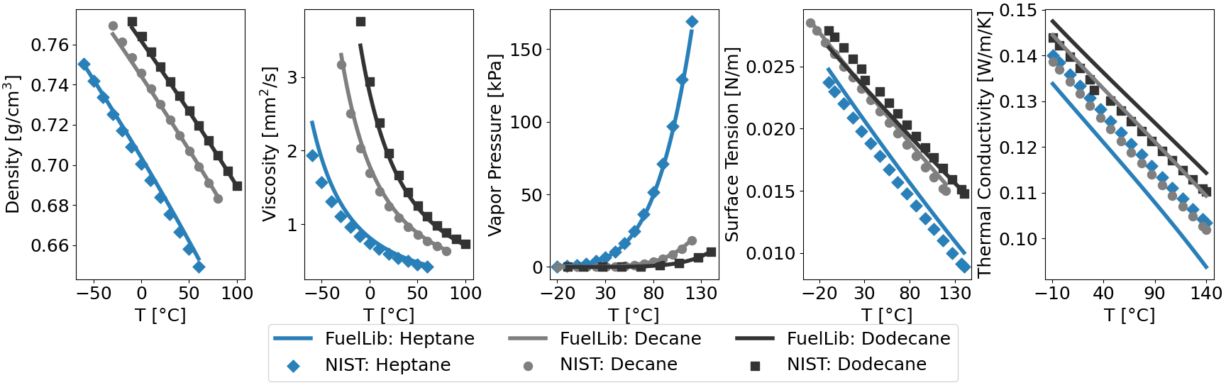
Fig. 1 Properties of heptane, decane, and dodecane against predictive data from NIST Chemistry WebBook.

Multi-Component Fuels

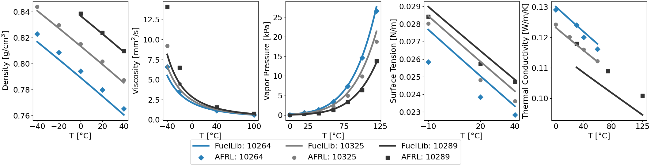
Fig. 2 Properties of conventional jet fuels JP-8 (POSF10264), Jet A (POSF10325), and JP-5 (POSF10289) against data from the Air Force Research Laboratory[5]. Note that the data sets for thermal conductivity are very inconsistent, but they typically show linear decreases in thermal conductivity with temperature.

Fuel Blends

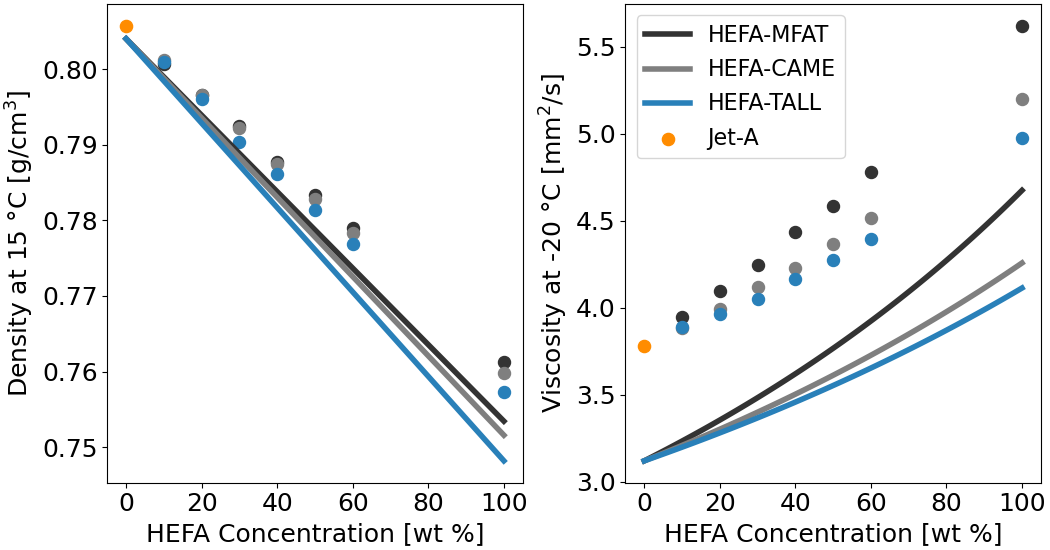
Fig. 3 Properties of three HEFA fuels produced from different feedstocks (camelina, tallow, and mixed fat) blended with Jet-A. Measurement and GCxGC data from Vozka et al.[6].

References

[1] (1,2,3,4,5,6,7,8,9,10,11)

Leonidas Constantinou and Rafiqul Gani. New group contribution method for estimating properties of pure compounds. AIChE Journal, 40(10):1697–1710, October 1994. URL: https://aiche.onlinelibrary.wiley.com/doi/10.1002/aic.690401011 (visited on 2024-07-08), doi:10.1002/aic.690401011.

[2] (1,2,3,4,5)

Leonidas Constantinou, Rafiqul Gani, and John P. O’Connell. Estimation of the acentric factor and the liquid molar volume at 298 K using a new group contribution method. Fluid Phase Equilibria, 103(1):11–22, January 1995. URL: https://linkinghub.elsevier.com/retrieve/pii/037838129402593P (visited on 2024-07-08), doi:10.1016/0378-3812(94)02593-P.

[3]

Meredith Colket, Joshua Heyne, Mark Rumizen, Mohan Gupta, Tim Edwards, William M. Roquemore, Gurhan Andac, Randy Boehm, Jeffery Lovett, Randy Williams, Jamey Condevaux, David Turner, Nader Rizk, Julian Tishkoff, Chiping Li, Jeff Moder, Daniel Friend, and Vaidya Sankaran. Overview of the National Jet Fuels Combustion Program. AIAA Journal, 55(4):1087–1104, April 2017. URL: https://arc.aiaa.org/doi/10.2514/1.J055361 (visited on 2025-01-28), doi:10.2514/1.J055361.

[4]

James T. Edwards. Reference Jet Fuels for Combustion Testing. In 55th AIAA Aerospace Sciences Meeting. Grapevine, Texas, January 2017. American Institute of Aeronautics and Astronautics. URL: https://arc.aiaa.org/doi/10.2514/6.2017-0146 (visited on 2025-01-17), doi:10.2514/6.2017-0146.

[5] (1,2)

James T. Edwards. Jet Fuel Properties. Technical Report AFRL-RQ-WP-TR-2020-0017, Air Force Research Laboratory, Wright-Patterson Air Force Base, OH 45433, 2020. URL: https://apps.dtic.mil/sti/pdfs/AD1093317.pdf.

[6] (1,2)

Petr Vozka, Pavel Šimáček, and Gozdem Kilaz. Impact of HEFA Feedstocks on Fuel Composition and Properties in Blends with Jet A. Energy & Fuels, 32(11):11595–11606, November 2018. URL: https://pubs.acs.org/doi/10.1021/acs.energyfuels.8b02787 (visited on 2025-06-27), doi:10.1021/acs.energyfuels.8b02787.

[7]

T.L. Nielsen. Molecular Structure Based Property Prediction, 15-point Project Department of Chemical Engineering. Technical University of Denmark Lyngby, 1998.

[8] (1,2,3,4,5,6)

Bruce E. Poling, John M. Prausnitz, and John P. O’Connell. The properties of gases and liquids. McGraw-Hill international editions Chemical engineering series. McGraw-Hill, New York, NY, 5. ed edition, 2001. ISBN 978-0-07-011682-5 978-0-07-118971-2. URL: https://www.accessengineeringlibrary.com/content/book/9780070116825?implicit-login=true.

[9] (1,2)

D. S. Viswanath and Dabir S. Viswanath. Viscosity of Liquids: Theory, Estimation, Experiment, and Data. Physica-Verlag NetLibrary, Inc. [distributor], Heidelberg Boulder, 2007. ISBN 978-1-4020-5482-2.

[10] (1,2,3,4,5,6)

Pavan B. Govindaraju and Matthias Ihme. Group contribution method for multicomponent evaporation with application to transportation fuels. International Journal of Heat and Mass Transfer, 102:833–845, November 2016. URL: https://linkinghub.elsevier.com/retrieve/pii/S0017931016309887 (visited on 2024-07-01), doi:10.1016/j.ijheatmasstransfer.2016.06.079.

[11] (1,2)

Harold G. Rackett. Equation of state for saturated liquids. Journal of Chemical & Engineering Data, 15(4):514–517, October 1970. URL: https://pubs.acs.org/doi/abs/10.1021/je60047a012 (visited on 2024-08-14), doi:10.1021/je60047a012.

[12] (1,2)

Tomoyoshi Yamada and Robert D. Gunn. Saturated liquid molar volumes. Rackett equation. Journal of Chemical & Engineering Data, 18(2):234–236, April 1973. URL: https://pubs.acs.org/doi/abs/10.1021/je60057a006 (visited on 2024-08-02), doi:10.1021/je60057a006.

[13] (1,2,3)

Byung Ik Lee and Michael G. Kesler. A generalized thermodynamic correlation based on three‐parameter corresponding states. AIChE Journal, 21(3):510–527, May 1975. URL: https://aiche.onlinelibrary.wiley.com/doi/10.1002/aic.690210313 (visited on 2024-08-09), doi:10.1002/aic.690210313.

[14] (1,2,3)

D. Ambrose and J. Walton. Vapour pressures up to their critical temperatures of normal alkanes and 1-alkanols. Pure and Applied Chemistry, 61(8):1395–1403, January 1989. URL: https://www.degruyter.com/document/doi/10.1351/pac198961081395/html (visited on 2024-11-11), doi:10.1351/pac198961081395.

[15] (1,2)

James R. Brock and R. Byron Bird. Surface tension and the principle of corresponding states. AIChE Journal, 1(2):174–177, June 1955. URL: https://aiche.onlinelibrary.wiley.com/doi/10.1002/aic.690010208 (visited on 2025-04-14), doi:10.1002/aic.690010208.

[16]

R. F. Curl and Kenneth Pitzer. Volumetric and Thermodynamic Properties of Fluids—Enthalpy, Free Energy, and Entropy. Industrial & Engineering Chemistry, 50(2):265–274, February 1958. URL: https://pubs.acs.org/doi/abs/10.1021/ie50578a047 (visited on 2025-04-14), doi:10.1021/ie50578a047.

[17]

Kenneth S. Pitzer, Gilbert Newton Lewis, and Merle Randall, editors. Thermodynamics. Mc-Graw-Hill Series in advanced chemistry. McGraw-Hill, New York, 3. ed edition, 1995. ISBN 978-0-07-050221-5 978-0-07-113809-3.

[18]

Kenneth G. Harstad, Richard S. Miller, and Josette Bellan. Efficient high‐pressure state equations. AIChE Journal, 43(6):1605–1610, June 1997. URL: https://aiche.onlinelibrary.wiley.com/doi/10.1002/aic.690430624 (visited on 2025-04-14), doi:10.1002/aic.690430624.

[19]

James Kendall and Kenneth Potter Monroe. THE VISCOSITY OF LIQUIDS. II. THE VISCOSITY-COMPOSITION CURVE FOR IDEAL LIQUID MIXTURES. $^\textrm 1$. Journal of the American Chemical Society, 39(9):1787–1802, September 1917. URL: https://pubs.acs.org/doi/abs/10.1021/ja02254a001 (visited on 2024-08-13), doi:10.1021/ja02254a001.

[20]

Svante Arrhenius. Über die Dissociation der in Wasser gelösten Stoffe. Zeitschrift für Physikalische Chemie, 1U(1):631–648, February 1887. URL: https://www.degruyter.com/document/doi/10.1515/zpch-1887-0164/html (visited on 2024-08-13), doi:10.1515/zpch-1887-0164.

[21]

Esaú A. Hernández, Gabriela Sánchez-Reyna, and Jorge Ancheyta. Evaluation of mixing rules to predict viscosity of petrodiesel and biodiesel blends. Fuel, 283:118941, January 2021. URL: https://linkinghub.elsevier.com/retrieve/pii/S0016236120319372 (visited on 2024-08-09), doi:10.1016/j.fuel.2020.118941.

[22]

J.A. Hugill and A.J. Van Welsenes. Surface tension: a simple correlation for natural gas + conensate systems. Fluid Phase Equilibria, 29:383–390, October 1986. URL: https://linkinghub.elsevier.com/retrieve/pii/0378381286850385 (visited on 2025-04-14), doi:10.1016/0378-3812(86)85038-5.